Contents
- The Basics
- Decision Trees
- Naive Bayes
- K-nearest Neighbours
- Linear Regression
- Robust Regression
- Clustering
- Principle Component Analysis (PCA)
- Linear Classification (+ Perceptron)
- The Kernel Trick
- MLE and MAP estimation
- Recommender Systems
- Neural Networks
- Ensemble Methods
For reference: these chapters are where I know what's going on: \[ 1、2、3、4、5、6、7、8、9、10\sim、13 \] And these uh nah. \[ 11、12、14 \]
\( \renewcommand{\vec}{\mathbf} \renewcommand{\epsilon}{\varepsilon} \DeclareMathOperator*{\argmax}{argmax} \DeclareMathOperator*{\argmin}{argmin} \def\xtrain{{\vec{x}_i}} \def\xtest{{\vec{\tilde{x}}_i}} \def\ytrain{{y_i}} \def\ytest{{\tilde{y}_i}} \def\ypred{{\hat{y}_i}} \def\yhat{{\hat{y}}} \def\wtrans{{\vec{w}^\top}} \def\bb#1{{\mathbb{#1}}} \def\x{{\vec{x}}} \def\X{{\vec{X}}} \def\w{{\vec{w}}} \def\W{{\vec{W}}} \def\y{{\vec{y}}} \def\Y{{\vec{Y}}} \def\t{{^\top}} \def\z{{\vec{z}}} \def\Z{{\vec{Z}}} \def\v{{\vec{v}}} \def\lra{{\longrightarrow}} \def\lla{{\longleftarrow}} \newcommand{\fr}{\frac} \newcommand{\vecu}{\underline} \newcommand{\rm}{\textrm} \newcommand{\bb}{\mathbb} \newcommand{\nm}{\overline} \newcommand{\tl}{\tilde} \)The Basics
Introduction
Machine Learning is the process of getting machines to learn to model stuff, that is, given experiences E to learn from, a set of tests T to measure against, for which we measure a performance P.
Patterns are learned from features, qualities that describe the data, which change depending on the data in question.
Input -> Extracting features (manual) -> Training and classification -> Results
Getting the machine to extract features itself is called representation learning, and is generally used in deep neural networks.
Recap
Machine learning takes basis on probability (and a lot of stats) - especially joint probability distributions (like \(p(A, B)\)).
Recall:
- The marginalisation rule \(p(A) = \sum\limits_{\forall x} p(A, B=x)\)
- Random Variables X, with an event \(X = x\) which occurs with some probability, the sum of all possible events is 1.
- Conditional probability \(p(A|B) = \frac{p(A,B)}{p(B)} \)
- Bayes Rule \(p(A|B) = \frac{p(B|A)p(A)}{p(B)}\)
Datasets are collections of samples - the range of values are limited and probably in some sort of distribution, which can take many forms, such as uniform (straight line) or gaussian/normal (bell curve).
Datasets can have a mean \(\mu\) and standard deviation \(\sigma^2\) -- variance is stddev-squared.
Distribution Functions
Probability density (PDF): probability of observing a value, i.e. \(p(X = x)\) \[ p(x|\mu, \sigma^2 ) = \frac{1}{\sqrt{2\pi \sigma^2}} \exp(-\frac{(x-\mu)^2}{2\sigma^2}) \]
Cumulative density (CDF): probility of observing ≤ the value \(p(X \leq x)\) \[p(X \leq x|\mu, \sigma^2) = \int_0^x \textrm{(curve)} dx\]
Expectation, the expected value, is denoted \(\mathbb{E} \), and given as \[\mathbb{E}[x] = \sum_{\forall x} p(X = x) \cdot x\]
Notation: the module uses standard notations for everything: \
Scalar
\(x\): lowercase (or upper case) letter.
Column Vector
\(\vec{x}\): bold lowercase letter. Vectors are always columns, so row vectors are always represented as \(\vec{x}^\top\). Dot products between vectors are often represented \(\vec{w}^\top \vec{x}\) (a matrix multiplication), though I may also use \(\vec{w} \cdot \vec{x}\)
Matrix
\[\vec{X} = \begin{bmatrix} x_{11} & x_{12} \\ x_{21} & x_{22} \end{bmatrix}\] Upper case bold letter. If a matrix is symmetric, \(\vec{X}^\top = \vec{X} \).
Supervised learning is when both questions and answers are given, and the model has to learn to predict answers from samples.
Unsupervised learning is when no answers are given, and the model has to find relationships between samples.
General Data Notation
Samples are stored in a matrix, generally denoted \(\vec{X}\), where each row is a sample, a feature vector, and each column is an individual feature. \(\vec{X} \in \bb{R}^{n \times d}\), which means that X has \(n\) rows (for n samples) and \(d\) columns (for d features/dimensions)
- \(\vec{x}_i\) is a sample row, represented as a column (as a row, it is consistently denoted \(\vec{x}_i^\top\)).
- \(\vec{x}_j \) is a column of features.
- \(x_{ij}\) is feature \(j\) of column \(i\).
Labels are stored in vector \(\vec{y}\), \(y_i\) being the label for an \(\vec{x}_i\). This is also called the ground truth
Given a new sample \(\tilde{\vec{x}}_i\) (tilde represents test data), we can make a prediction \(\hat{y}_i\) for it (the hat represents predicted).
Decision Trees
The Scenario
Suppose you start to frequently get upset stomachs, and worry that it is due to an allergy that you don't know about, perhaps to one food, perhaps to a combination. So, you decide to keep a food diary, detailing what allergen-inducing foods you consume each day, in what amounts, and whether or not you had an upset stomach that day.
| Milk | Eggs | Peanuts | Crustaceans | Upset? |
|---|---|---|---|---|
| 0.3 | 0.2 | 0 | 0.7 | 1 |
| ... | ... | ... | ... | ... |
This is a type of supervised learning problem, we have our features (foods and amounts) and our classes (upset stomach / not), and want to train a classification algorithm to predict things.
The Decision Tree
A simple classifier is a decision tree
A decision tree is essentially a nested series of if-elif-elses, that split the dataset up -- these are splitting rules.

Our aim is then to find these rules, which can be done recursively:
Stumps
The most basic decision tree is a stump. A stump is just one single splitting rule, the smallest possible tree.
To find a tree, we must first find a stump, but we need to find the stump that splits the best. How? With some scoring metric.
Ex. Could use plain accuracy, take a rule like eggs > 0.2 and set a True and False coming off it - we now have a stump that can predict data. Pick the rule with the highest amount of data correctly predicted.
In our stump finding then, our training error would be just the percentage of \(\hat{y}_i \neq y_i\), i.e. the accuracy.
Greedy Recursive Splitting
A stump, however, can only split on one thing, and if we have \(d\) features we kinda want more splits, otherwise we're only ever using one of the features.
A common algorithm is greedy recursive splitting (GRS), which goes as follows:
- Find a stump with the best score metric, and split the dataset into two smaller ones at that stump. (The new split datasets would probably still have a mix of \(y\)s, but hopefully are much more uniform than before)
- Recurse: "fit" (find) a new stump onto each of the smaller datasets, this is linked onto the previous stump.
- Repeat until accuracy threshold reached (or depth reached, or some other limit. Accuracy can be 100%, but this may result in an overcomplex tree and not always be helpful, "overfitting").
Currently, we have accuracy as a possible metric, but this may not always be good, especially when there's multiple possible stumps that increase accuracy by the same amount, or the data is spread in such a way that a single line does not do much for accuracy.
A better way is if we could prioritise variance reduction, some sort of ... information gain:
Entropy
Entropy of labels is essentially the randomness of their values. For a total of \(C\) categories, this can be calculated as \[E = -\sum_{c=1}^C p_c \cdot \log_2 (p_c)\] where \(p_c\) is the proportion of \(c\) out of all total labels in that (sub)set. Note that \(0\log_2 0\) is defined to just be 0.
A lower entropy (min. 0) means less randomness, which is better. A higher entropy (max. \(log_2 C\), or 1 for binary classes) is worse.
Information Gain
The principle of Information Gain (IG), is that we want the biggest difference in entropy pre-split to post-split.
For a single rule, we can split the set of \(n\) elements into \(n_{yes}\) (for the samples that match the rule) and \(n_{no}\) for the ones that don't. Thus IG is defined \[ IG = E(\vec{y}) - \frac{n_{yes}}{n} E(\vec{y}_{yes}) - \frac{n_{no}}{n} E(\vec{y}_{no}) \] i.e the entropy of combined labels \(\vec{y}\) minus the entropy of split labels individually.
The higher this difference is, the better the split is.
The final algorithm (the ID3 algorithm, is given as follows:)
Overfitting and Learning Theory
If we have 100% accuracy on our training data, this does not imply that we have 100% accuracy on any new test data.
- Test Accuracy is the accuracy on new data
- Overfitting or Optimisation Bias is high accuracy on training data but low on test data
- Underfitting is low accuracy on training data.
We naturally want the right amount of fitting, but this is difficult.
We can use a test/verification set \(\tilde{\vec{X}}\) to verify, but we must ensure that we do not train using the verification set.
The IID Assumption (Independent and Identically Distributed) states that we assume that the training data is a good representation of all data - that is, it has the same distribution as test data.
Whilst this is often not true, it is generally a good assumptuion.
Learning Theory gives us a metric for measurement, \(E_{approx}\) the approximation error, the error between training and testing: \[E_{test} = E_{approx} + E_{train}\] where \(E_{approx} = E_{test} - E_{train}\). If this is small, then we can say that the training data is good for test data. It tends to go down as the training set gets larger, and up as the model gets more complex (and thus overfit).
However, this approximation error leads to a fundamental tradeoff: minimise \(E_{approx}\) whilst minimising \(E_{train}\): make the model not overfit whilst having it be fit as well as possible.
Validation
Usually, we split a training set into two: a larger x_train (the "training set"), and a smaller x_test, what's called the validation (or colloquially test) set.
Once we train on x_train, we can compute the accuracy of predicting x_test, and use this to adjust our model, such as manually setting hyperparameters.
Hyperparameters are settings in a model which we do not learn. For decision trees, this may be the maximum depth of the tree, or the accuracy threshold. For more complex models like Neural Networks, the entire architecture is hyperparameter, whilst the weights and biases are learned, regular parameters.
With simpler models, it is often good to train it multiple times with different hyperparameter settings (like tree depth), and see which one minimises both training error and approximation error the best.
Sometimes, once hyperparameters are set, a model is trained again, with x_test merged back into the training set (no validation).
That said, we may end up overfitting the validation set. If we search too many and too specific hyperparameters, we may end up finding one that's really good for the validation set, but not so good for any new data.
- Optimisation bias increases as we search for more model configurations
- It decreases as the training data gets larger.
This leads to another fundamental tradeoff: increasing validation size means our model is less likely to be overfit. However, increasing validation size decreases test size, which makes our model train less well.
Cross Validation
Validation takes from test data, if test data is precious and hard to get, we may not want to waste it.
K-fold cross validation gives a good estimate without wasting too much data.
For K folds, we train K times, each time taking \(\frac{1}{k} \) of \(\vec{X}\) as validation, and the rest \(\frac{k-1}{k}\) as train. The average validation accuracy is taken as the overall accuracy
Leave One Out (LOO) is a special type of K-fold validation where \(k = n\).
Naive Bayes
The Scenario
You want to filter out which emails incoming are spam or not. For this, you've collected many, many emails, and labelled them correctly.
Your features are going to be keywords in emails, thus, \(x_{ij} = 1\) if the word \(j\) is in email \(i\).
Probabilistic Classification
Traditional filtering/classification methods used something called Naive Bayes - a probability based classifier based on bayes rule.
The idea is, we want to model \(p(y_i | \vec{x}_i)\): probability of it having that label, given those features. If \(y_i\) was binary, then we could classify \(\vec{x}_i\) as true if \(p(y_i | \vec{x}_i) > p(\lnot y_i | \vec{x}_i)\).
Given bayes rule, and a y-label \(spam, \; \lnot spam\), we can use Bayes rule: \[ p(spam | \vec{x}_i) = \frac{p(\vec{x}_i | spam)p(spam)}{p(\vec{x_i})} \] (And similar for non-spam.) \(p(\vec{x}_i)\) is the probability that email \(i\) has those words in it.
\(p(spam)\)
Very easy to calculate, it's just the proportion of positive to all \(p(spam) = \frac{\sum spam}{n}\)
\(p(\vec{x})_i\)
Very difficult to calculate, however due to the classification rule we use: \begin{align} p(y_i | \vec{x}_i) &> p(\lnot y_i | \vec{x}_i) \\ \implies \frac{p(\vec{x}_i | y_i)p(y_i)}{p(\vec{x_i})} &> \frac{p(\vec{x}_i | \lnot y_i)p(\lnot y_i)}{p(\vec{x_i})} \\ \implies p(\vec{x}_i | y_i)p(y_i) &> p(\vec{x}_i | \lnot y_i)p( \lnot y_i) \end{align} We can just ignore the term.
\(p(\vec{x_i} | spam)\)
Equals \(\frac{\sum \textrm{ spam emails with } \vec{x}_i}{\sum spam}\), which is very hard to work out, and no easy workaround:
Make a conditionally independent assumption: assume the occurence of every \(x_{ij}\) is independent from every other \(x_{ij'}\). This is why the Bayes is naive.
Thus \(p(\vec{x_i} | spam) \approx \prod\limits_{j=1}^{d} p(x_{ij} | spam)\).
Whilst this is rarely true, it is in some cases a good enough approximation.
More generally, when predicting data, we find the class \(c\) of \(y\) that has the highest probability given an \(\tilde{\vec{x}}_i\).
There is one other problem: when data is missing from our set but we still want to account for it. For example, if you want to detect the chance an email containing "millionaire" is spam, but none of your collected spam emails have that word.
We can use laplace smoothing to account for this: if a feature \(x_{ij}\) has \(k\) possible values, for some \(\beta \in \bb{R}\): \[ \frac{p(x_{ij} = e) + \beta}{\textrm{total }+ k\beta} \] i.e. add a fake value to the proportion of emails that have the feature we want, but add everything else in the same proportion to the total, so proportions are kept consistent.
For binary features (and \(\beta = 1\)), we can do \[ \frac{ \#\textrm{spam with 'millionaire' } + 1 }{ \#\textrm{total spam } + 2 } \]
K-Nearest Neighbours
The models looked at previously were parametric -- that is, they had a fixed number of parameters (fixed by hyperparmameters, the model size is O(1) w.r.t. data size)
K-nearest neighbours (KNN) is in the class of non-parametric models, that is, the larger the dataset, the larger the model gets.
KNN is a classification model, that works by taking a new point \(\vec{\tilde{x}_i}\) and comparing it to its \(k\) "closest" neighbours from the training set, classifying it into the majority category.
It works off the Lipschitzness Assumption, that if two feature vectors are "close", they are likely to be similar.
This closeness is most commonly done using L2 Norm: euclidean distance \(\lVert \vec{x}_i - \vec{\tilde{x}}_i \rVert\).
Note that euclidean distance is often written \(|\vec{a}|\) in mathematics, or with double bars and an explict L2-norm indicator \(||\vec{a}||_2\), seen in ML.
The way KNN calculates its \(k\) nearest neighbours is simply by calculating euclidean distance to all \(\vec{x} \in \vec{X}\) and finding the closest ones. Thus,
- There's no traditional learning (lazy learning), simply store the data
- Non parametric size, size \(\propto O(nd)\) for \(n\) samples and \(d\) dimensions
- Predicting is expensive, \(O(ndt)\) for \(t\) test samples
A Norm is a way of "calculating distance", so to say. There are three (maybe four) common norms:
| L2 | L1 | (L0) | L\(\infty\) |
|---|---|---|---|
| \[\lVert \vec{r} \rVert_2 = \sqrt{r_1^2 + r_2^2}\] | \[\lVert \vec{r} \rVert_1 = |r_1| + |r_2|\] | \[\lVert \vec{r} \rVert_0 = nz(r_1) + nz(r_2)\] \[\textrm{s.t. } nz(x) = \begin{cases} 1 & x \neq 0 \\ 0 & x = 0 \end{cases}\] | \[\lVert \vec{r} \rVert_\infty = \max(|r_1|, |r_2|)\] |
| Euclidean distance | Manhattan distance | Counts nonzero values | Max |
| Emphasises larger values | All values are equal | (Not actually a norm) | Only the largest component matters |
The numbers are given with reason: the \(L_p\) norm for \(p\geq 1 : \lVert \vec{x} \rVert_p = \sqrt[\fr{1}{p}]{ \sum\limits_{j=1}^d |x_j|^p }\)
A 1NN classifier is just nearest neighbour, every point defines a cell, within which everything belongs to its category (a "voronoi tesselation"). Boundaries between cells are decision boundaries, assignment here can be arbitrary.

Test Errors, and Optimal Bayes
We can compare the error of a KNN (or 1NN) classifier against the Optimal Bayes Classifier.
Recall Naive Bayes: we assume that all features are independent. Optimal Bayes is a theoretical Bayes classifier that does not make this assumption.
Optimal Bayes will then predict \(\hat{y_i} = \argmax\limits_{y_i} p(y_i | \vec{x}_i)\), taking into account all conditional probabilities.
Note that Optimal Bayes is not a perfect classifier, it still has an error \(\epsilon_{bayes} = 1 - p(\hat{y}_i | \vec{x}_i)\), but this error is agood lower bound on potential error of classifier.
Claim. For a 1-NN classifier, as \(n \longrightarrow \infty\) its error \(\epsilon_{1NN} \longrightarrow 2\epsilon_{bayes}\)
Proof. Assume a two class 1NN, with classes + and -.
- With more samples, the distance between \(\vec{\tilde{x}}_i\) and its closest neighbour tends to 0 (imagine the space filling up with points.)
- We want to find the probability that it is a false classification, \(p(\hat{y} \neq \tilde{y} | \vec{\tilde{x}})\)
- If positive \(p(+|\vec{x}_i)\), the classifier can predict rightly with probability \(p(+|\vec{x}_i) p(+|\vec{\tilde{x}}_i)\) or wrongly \(p(+|\vec{x}_i) (1-p(+|\vec{\tilde{x}}_i))\)
- Similarly if negative it can get it correct \((1-p(+|\vec{\tilde{x}}_i))(1-p(+|\vec{\tilde{x}}_i))\) or wrong \( (1-p(+|\vec{\tilde{x}}_i))p(+|\vec{x}_i)\)
- Note that there are two false probabilities, \begin{align} \epsilon_{1NN} &= p(\hat{y}_i|\vec{x}_i) (1-p(\hat{y}_i|\vec{\tilde{x}}_i)) + (1-p(\hat{y}_i|\vec{\tilde{x}}_i))p(\hat{y}_i|\vec{x}_i) \\ &\geq (1-p(\hat{y}_i)|\vec{x}_i) + (1-p(\hat{y}_i)|\vec{x}_i) \pod{\textrm{ignore tilde}} \\ &\geq 2(1-p(\hat{y}_i)|\vec{x}_i)\\ & \geq 2\epsilon_{bayes} \end{align} $$\tag*{$\Box$}$$
The error of k-NN classification tends to \((i+\sqrt{\frac{2}{k}} ) \epsilon_{bayes}\).
The Curse of Dimensionality (Runaway Exponents)
In practice though, we cannot get that good of an error. Because we need a very large \(n\), to get a crowded enough feature space.
In 2D, we can imagine our feature space to be a circle, with area \(O(r^2)\), thus \(n = O(r^2)\). In 3D, this increases to \(O(r^3)\) and realistically ML has way more than 3 dimensions, and so the amount of data we need \(n \approx c^d\), for \(d\) dimensions and a constant \(c\).
We also have an upper bound error: the constant classifier, that always returns the most common label: simply set \(k=n\). Naturally, our model is only a success if it does (significantly) better than n-NN.
Linear Regression
Get ready for some Linear Algebra
Classification predicts best classes, when labels are discrete. Regression predicts best fit, when labels are continuous.
Linear Regression is a tool for modelling linear relationships - literally a line of best fit.
For training data \(\vec{X} \), labels \(\vec{y} \), we can define a regression function \(h:\vec{X} \longrightarrow \vec{y}\) as \[\hat{y}_i = h(\vec{x}_i) = \vec{w} \cdot \vec{x_i}\] Note that this is literally \(y = mx + c\) but without the \(+c\). \(\vec{w} \) (the weights) is the slope of the line, and this is what we want to find.
We find this by minimising a loss function, a function that describes the error of our predictions w.r.t. the training data.
The most common loss function used is mean squared error (MSE): \[ \mathcal{L}(h) = \frac{1}{n} \sum_{i=1}^n (h(x_i | w) - y_i) ^ 2 \] Basically, sum of the difference between predicted and actual \(y\), squared. Thus we find \(\argmin\limits_\vec{w} \cal{L}(h)\). This is known as finding least squares.
Note that the loss function can be denoted \(\cal{L}(\cdot)\) or just \(f(\cdot)\), I often prefer the former when note taking but you see the latter used quite often.
The loss function is quadratic in \(\vec{w} \) (in this case), and so we can find a minimum easily.
Note. Minimising \(\frac{1}{n} \sum(\cdots)\) is the same as minimising \(\sum(\cdots)\) or any other constant multiplier. \(1/2\) is often used for convenience of differentiation.
1D Regression
1D regression is the easiest case. We have a function \(\cal{L}(w) = \frac{1 }{2 } \sum\limits_{i=1}^n (wx_i - y_i)^2\) for a scalar \(w\). \begin{align} \therefore \cal{L}(w) &= \frac{1 }{2 }\sum_{i=1}^n (w^2x_i^2 - 2wx_iy_i + y_i^2) \\ &= \frac{w^2 }{2} (\sum x_i^2) - \frac{2w }{2 } (\sum x_i y_i) + \frac{1}{2} (\sum y_i^2) \\ &= \frac{a}{2} w^2 - bw + c \end{align} (Since the sum terms are constant)
\(\cal{L}' (w) = wa-b\), set to 0 and solve for \(w\), \(w = \frac{b}{a}\)
We can also use the second derivative to make sure it is a minimum.
This finds the best \(w\) ... for a line \(\hat{y}_i = wx_i\) that passes through 0, because we haven't accounted for bias.
Bias, Extending Dimensions
A bias is an extra constant added on, that shifts the result up or down. For 1D, we change the equation to \(\hat{y}_i = wx_i + w_0\) where \(w_0\) is the bias.
We can add bias by changing basis: we make a "fake feature", with 1 for all the values: \[ \vec{X} = \begin{bmatrix} x_i \\ x_2 \\ \vdots \\ x_n \end{bmatrix} \longrightarrow \vec{Z} = \begin{bmatrix} 1 & x_1 \\ 1 & x_2 \\ \vdots &\vdots \\ 1 & x_n \end{bmatrix} \] Thus, we are effectively using \(\vec{Z}\) as our feature set, and have to solve \[ y_i = v_1 z_{i1} + v_2 z_{i2} \equiv w_0 + w_1x_i\] Note that because we changed basis, our transformed features are now denoted \(z\) and our transformed wieghts are denoted \(v\).
This creates 2D linear regression.
When we learn in 1D, we are fitting a line of best fit. In 2D, then, we are fitting a plane of best fit. And the dimensions of the (hyper)plain just increases.
For \(d\) features (ignoring bias), we have a \begin{align} \ypred &= w_1 x_{i1} + \cdots + w_d x_{id} \\ &= \sum_{j=1}^d w_j x_{ij} \\ &= \vec{w}^\top \xtrain \equiv \vec{w} \cdot \xtrain. \end{align} The loss is then the MSE: \[ \cal{L} = \frac{1}{2} \sum_{i=1}^n (\wtrans \xtrain - y_i)^2 \]
Whilst finding derivatives for this can be difficult from a partial differentiation perspective, we can actually differentiate matrices fine, which we'll soon see.
Matrix Magic
It is probably good now to mention the dimensions of the data.
- \(\vec{y}: n \times 1 \)
- \(\xtrain : d \times 1\)
- \(\vec{X} : n \times d\); can be thought of as rows of \(\xtrain^\top\) (transposed so coln -> row)
A single prediction \(\ypred = \vec{w} \cdot \xtrain\). All \(n\) samples can then be gotten from \(\vec{\hat{y}} = \vec{X} \vec{w}\).
We say that \(\vec{\hat{y}} - \vec{y} = \vec{r}\), the residual vector, and being the error difference, we can write MSE using it: \[ \cal{L}(\vec{w}) = \frac{1}{2} \lVert \vec{r}^2 \rVert^2 = \frac{1 }{2 }\lVert \vec{X} \vec{w} - \vec{y} \rVert^2 \]
Thus we can find an error using matrix calculus; a symbol will be used here called "nabla" \(\nabla\), which represents multi-dimensional differentiation. For the case of vectors, think of deriving each term element-wise.
\begin{align} \implies \cal{L}(\vec{w}) &= \frac{1 }{2 } \vec{w}^\top \vec{X}^\top \vec{X} \vec{w} - \vec{w}^\top \vec{X}^\top \vec{y} + \frac{1 }{2 }\vec{y}^\top \vec{y} \\ &= \frac{1 }{2 }\vec{A w^\top w} - \vec{b w^\top} + \frac{1 }{2 }c \pod{\vec{X^\top X, X^\top y, y^\top y} \textrm{ are constant}} \\ \nabla \cal{L} (\vec{w}) &= \nabla(\frac{1 }{2 }\vec{A w^\top w}) - \nabla (\vec{bw^\top}) + \nabla(\frac{1 }{2 }c) \\ &= \vec{Aw-b}. \pod{\textrm{if } \vec{A} \textrm{ symmetric}} \end{align}Then, all we need to find is \(\vec{Aw - b} = 0\), or equivalently \(\vec{X^\top X w - x^\top y} = 0\)
\[ \implies \vec{w = (X^\top X)}^{-1} \vec{X^\top y}. \]MSE has some issues however.
- MSE is sensitive to outliers, as large differences are empasised more greatly.
- Finding a model can be memory and time intensive - there are a lot of large matrix multiplications, and large systems of equations.
- May extrapolate: predicting values outside of the measured range.
- Solution may not be unique: colinear features, where 2 features are identical for all samples, which means that both, say, \(y_i = w_1 x_1 + w_2 x_2 \equiv y_i = 0 x_1 + (w_1 + w_2)x_2\), are valid solutions.
- And finally, linear regression assumes a linear relationship.
Note. The term convex refers to functions with a shape like \(\cup, \cap\), meaning they have only one minima (or maxima). It is easy to optimise these functions (not so for non-convex ones)
Polynomial Regression
Often, there is not a linear relationship.
So what do we do? Well, we can very easily "hijack" least squares linear regression to do polynomial regression, in the same method that we use to add a bias.
Suppose again 1D samples \(\vec{X}\), that we suspect has a polynomial relationship to \(\vec{y}\), we can also change the basis to account for squares:
\[ \vec{X} = \begin{bmatrix} x_i \\ x_2 \\ \vdots \\ x_n \end{bmatrix} \longrightarrow \vec{Z} = \begin{bmatrix} 1 & x_1 & x_1^2 \\ 1 & x_2 & x_2^2 \\ \vdots &&\vdots \\ 1 & x_n & x_n^2 \end{bmatrix} \]And would you look at that, we now have the squared features as a separate feature. Now simply fit a line \(\ypred = v_1 z_{i1} + v_2 z_{i2} + v_3 z_{i3}\).
We can also naturally extend this to higher polynomials. However, too high polynomials leads to overfitting - whilst training error may go down, test error goes up.
That is, fit new parameters \(\vec{V}\) on transformed featuers \(\vec{Z}\), by solving for \(\vec{ZZ^\top v = Z^\top y} \).
To predict on a validation set \(\vec{\tilde{X}}\), first transform it into the polynomial form \(\vec{\tilde{Z}}\), then do \(\vec{y = \tilde{Z} v }\).
L2 Regularisation
Training a regression model may produce excessively large weights.Exessively large weights are very sensitive, thus are more likely to be overfit -> penalise large weights.
L2 Regularisation is an extra bit we add to our MSE loss: \[ \cal{L}(\vec{w}) = \frac{1}{2} \lVert \vec{Xw - y}\rVert^2 + \frac{\lambda}{2}\lVert \vec{w} \rVert^2 \] Note the new \(\frac{\lambda}{2}\lVert \vec{w} \rVert^2 \) term. This new lambda parameter controls how much emphasis we want on small weights. A high \(\lambda\) means that we want small weights more than least squares, whereas \(\lambda = 0\) removes the penalty altogether.
\(\frac{\lambda}{2 }\) is done for ease of differentiation.
Furthermore, the derivative \(\nabla \cal{L}(\vec{w}) = \vec{X^\top X w - X^\top y + } \lambda \vec{w}\) solves for the equation \((\vec{X^\top X + \lambda I}) \vec{ w = X^\top y}\), and the matrix that multiplies into \(\vec{w}\) is always invertible.
Robust Regression
Outliers and Loss
As mentioned, MSE is greatly affected by outliers, as large deviations are emphasised more. Instead, we can use absolute error (instead of squared error) to de-emphasise large deviations.
Absolute (L1) loss is defined as \[ \cal{L}(\w) = \sum_{i=1}^n |\w\t \x_i - y_i| \]
Minimising L1 though is much harder, as the absolute function is non-differentiable at \(x=0\), and the gradient is not smooth.
This poses problems for our minimisation equations, problems that L2 doesn't. Thus, we want a loss function that gets the best of both worlds.
The Huber loss function is defined \[ \cal{L}(\w) = \sum_{i=1}^n h(\w\t \x_i - y_i) \] Where \[ h(r_i) = \begin{cases} \frac{1 }{2 }r_i^2 & |r_i| \leq \epsilon \\ \epsilon(|r_i| - \frac{1 }{2 }\epsilon) & \textrm{otherwise. } \end{cases} \] For a small number \(\epsilon\).
Huber function is differentiable, becoming \[ h'(r_i) = \begin{cases} r_i & |r_i| \leq \epsilon \\ \epsilon \cdot \textrm{sign}(r_i) & \textrm{otherwise} \end{cases} \] Where \(\textrm{sign}(x) = 1 \textrm{ if } x > 0 \textrm{ else } -1\).
Standardising Features
Standardising features involves rescaling features so that they're all proportional to each other.
In some cases, we don't need to -- for basic models like Bayes and Decision Trees, we don't need to change. For least squares, though weights may be different, fundamentally the model is still the same.
However, standardisation is important for KNN (as large numbers can skew distance unnecessarily) and for regularised least squares (as penalty must be proportional).
Data is standardised feature-wise; for each feature \(j\):
- Compute mean \(\mu_j = \frac{1}{n} \sum_{i=1}^n x_{ij}\)
- Compute standard deviation \(\sigma_j = \sqrt{ \frac{1 }{n} \sum_{i=1}^n (x_{ij} - \mu_j)^2 }\)
- Replace every \(x_{ij}\) by \(\frac{x_{ij} - \mu_j}{\sigma_j}\)
HOWEVER, when standardising test data, do not use test data mean/stdevs, because technically, we don't know test data, and our assumption is that the training set is a good representation of any new data.
Labels/targets/ground truths can also be standardised, in the same way.
Feature Selection and Regularisation
Sometimes, we have a lot of features, but only a few of them matter.
We'd like the model to learn which features of \(\X\) are important.
One way we can do this is to look at the trained weights \(\w\), and take all features \(j : |w_j| >\) a predifined threshold.
Unfortunately, this has some downsides:
- It struggles with coliniearily and may give wrong results then, as if \(x_1, x_2\) are coliniear, then \(w_1 x_1 + w_2 x_2 \sim (w_1 + w_2) x_1 + 0x_2\).
- May pick up irrelevant features which happen to cancel: given irrelevant \(x_a, x_b\), then \(0x_a + 0x_b \sim -1000x_a + 1000x_b\).
Alternatively we can use a tactic of search and score, by defining (or using a function) \(f\) that computes a "score" of how good this set of features is -- such as the loss function.
Of course, this risks overfitting, especially since we're iterating over all \(2^d\) subsets, the optimisation bias can be high.
Instead, we modify the loss function to add a complexity penalty, such as \[ \cal{L}(s) = \frac{1 }{2 }\sum_{i=1}^n (\w_s \cdot \x_{is} - y_i)^2 + \textrm{size}(s) \] for a subset of features \(s\). The size function counts the number of nonzero weights -- the L0 norm;
Our Loss score becomes \[ \cal{L}(\w) = \frac{1}{2} \lVert \X\w - \y \rVert^2 + \lambda \lVert \w \rVert_0 \] With a parameter lambda.
The problem is, L0 is not convex ... nor differentiable, whereas L2 was very nice indeed, so if we can find a best of both worlds:
Use the convex and (mostly) differentiable L1 loss: \[ \cal{L}(\w) = \frac{1}{2} \lVert \X\w - \y \rVert^2 + \lambda \lVert \w \rVert_1 \] Also called LASSO regularisation.
A sparse matrix has many zeros: this is a good sign of feature selection.
Both L0 and L1 (LASSO) prefer sparsity, whilst L2 (Ridge) doesn't.
Clustering
Introduction
Clustering is a type of unsupervised learning.
In unsupervised learning, we are given no labels, and have to infer the underlying "latent" structure.
This is especially useful for outlier detection, grouping, latent factor models (later), and visualisation, among others.
For clustering, we are trying to group data into clusters based on their "similarity", and discover the distribution of data.
Often this data is multimodal, where there are more than one "peak" in its distribution (vs, say, a normal distribution, which has one mode).
Some assumptions:
- The features \(\X = \{\x_1 \cdots \x_n\}\) are in euclidean space.
- \(\X\) can be grouped into \(K\) groups or clusters (this is a hyperparameter);
K-Means Clustering
Assuming that there are K clusters, and that each sample is close to a cluster centre. In the off chance you're like me and misread K-means, "means" refers to "averages" like of data, and not "methods".
We use a heuristic-based improvement: starting with initial random means, and iterate by:
- Fix means, optimise points. Assigning each \(\x_i\) to its closest mean.
- Fix points, optimise means. Recompute means
- Refine until convergence (the means do not move or do not move enough)
And our metric of goodness (i.e. loss function) will be defined as:
For cluster means \(\vec{m} \) and assignments \(\vec{r} \), the mean squared distance: \[ \cal{L}(\{\vec{m}\}, \{\vec{r}\}) = \sum_{i=1}^n \sum_{j=1}^K r_j^i \lVert \vec{m}_j - \x_i \rVert^2 \pod{r^i_j \in \{0,1\}} \] Where \(r^i_j\) of data \(i\) to cluster \(j\) is 1 if that data is assigned to that cluster, or 0 otherwise.
Note: thus each \(\x_i\) will have a \(\vec{r}\) being a one-hot-encoding of its cluster.
The way a sample is assigned to a mean \(k\) is via euclidean distance \(k_i = \argmin\limits_k \lVert \vec{m}_k - \vec{x}_i \rVert^2\)
And means are adjusted via \(\vec{m}_k = \dfrac{\sum_i r^i_k \x_i}{\sum_i r^i_k }\) -- we need to include \(r^i_k\) to ensure we don't include features not assigned to that mean currently.
While K-means' loss heuristic is non-convex (i.e. not guaranteed global minimum), we are guaranteed a local minimum, we won't diverge ever.
Some issues though:
- \(K\) is a hyperparameter - if you don't know how many there should be, welp, sucks for you.
- Each example can only be assinged to one cluster (fixable)
- May converge to sub-optimal groups (can use methods such as random restart, non-local split and merge to fix)
Soft K-means
Soft K-Means makes partial assigments -- a sample can have partial membership of two clusters. For example, if an \(\x\) is a point that is very close to mean A and further but still close to mean B, it could be given the assignment \(\vec{r} = \{A = 0.84, B = 0.16\}\), like a probability.
We also call this fuzzy k-means.
We must set that all assignments must sum to one, using an important function called softMax:
\[
r^i_k = \frac{\exp(-\beta \lVert \vec{m}_k -\x_i \rVert^2)}{
\sum\limits_{j=1}^K \exp(-\beta \lVert \vec{m}_j -\x_i \rVert^2))
}
\]
Where \(\exp(x)\) is the exponential function: \(e^x\).
\(\beta\) is the stiffness parameter, controlling how "soft" assignments are -- emphasising one main class or allowing a more even spread.
If you plot the softMax curve, the stiffness controls how steep the center bit is.
For Soft K-means, we alter the loss function slightly. We say that now \(r^i_j \in [0,1]\), that we can get a range of values. Then, for one mean the loss is \(\newcommand{\m}{\vec{m}} \m_l = \argmin_\m \sum\limits_{i=1}^n r^i_l \lVert \m - \x_i \rVert^2\), and overall \[ \cal{L}(\m) = \sum_{l=1}^n \vec{r}^i \lVert \m - \x_i \rVert^2 \]
This loss function is actually quadratic - there is a unique solution.
Said unique solution is given by solving the first derivative \(\nabla \cal{L} (\m) = \sum_{i=1}^n \vec{r}^i(2\m - 2\x_i).\)
What we can do with K-means is actually do a primitive form of data reduction - approximating the data onto a lower space. In this case, by replacing all data points with their closest means, we do vector quantisation, which has this effect.
Thus overall, the soft k-means algorithm is as thus:
- Assing points via \(r_k^i = \textrm{softMax}_\beta (\lVert \m_k - \x_i \rVert^2 \)
- Update points via \(\m_k = \dfrac{\sum_{i=1}^n r_k^i \x_i}{\sum_{i=1}^n r_k^i }\)
Principle Component Analysis (PCA)
Introduction
Principal Component Analysis is fundamentally about approximating a feature set in a lower-dimensional "latent space" or subspace. i.e. reduce the dimensions, to extract higher level features, or to store less data overall.
One can think about images: images are comprised of possibly hundreds or thousands of pixels, but we can extract larger regions, to act as "components" to reconstruct said image.
Latent Factor Models (LFMs) are ML models that convert data to latent spaces.
We call the original dataset \(\X\), and can call the transformed "latent" set \(\Z\).
One method of this is vector quantisation - by doing k-means and then replacing each feature with its mean, we have replaced a sample sized \(1 \times d\) (d features) with \(1 \times k\) (k means). Now of course, if \(k > d\), this is hardly helpful.
Instead, we want to somehow learn the basic components that make up a sample \(x\), and weight them appropriately to reconstruct the original sample (as well as possible).
PCA
The PCA algorithm takes an \(\X\), and produces two vectors, \(\Z, \W\), which are in the following form:

- \(\W\) are our principal components, the components needed to reconstruct the features of \(\X\), ranging from the most fundamental component at the top (the first row), to the least important component at the bottom. We have \(k\) of these.
- \(\Z\) are the weights that reconstruct \(\W\) into \(\X\) - each \(\x_i = \W\t \z_i\). One single feature of one sample, \(x_{ij} \) involves multiplying row \(i\) of Z with column \(j\) of W.
- \(k \leq d\). Note that if \(k \ll d\), we can save a lot of storage space. The proof is trivial and left as an excersise to the reader.
PCA is a linear reduction - it can't extract non-linear features on its own. It's essentially just doing a matrix factorisation.
PCA is also useful especially to visualise high-dimensional data, as we only live in 3D.
The Theory
[1] To do PCA, we must first center data. Given an \(\X = \{\x_1, \x_2, \dots, \x_d\}\), compute the mean of its features \[ \vecu{\mu} = \fr{1}{n} \sum_{i=1}^n \x_i \] and then take it away from \(\X\) row-wise; \(X - \vecu{\mu}\). I'm using underline vector notation for mu, since LaTeX doesn't boldface greek fonts.
[2] To solve PCA, we need to learn weights, and adjust based on reconstruction error. We can use MSE for this: \begin{align} \cal{L}(\W, \Z) &= \sum_{i=1}^n \lVert \W\t \z_i - \x_i \rVert^2 \\ &= \lVert \Z\W - \X \rVert^2_F \end{align} for two matrices, \(\W, \X\). Note the subscript F is the frobenius norm -- L2 norm but over matrices.
[3] The PCA objective function is non-convex -- it doesn't have a unique global minimum. This makes finding a solution hard.
We can enforce a few constraints on each row/component to help us reduce bias and redundancy:
- Normalisation: enforce \(\lVert \w_c \rVert = 1\)
- Orthogonality: enforce \(w_c \cdot w_{c'} = 0 \forall c \neq c'\)
- Sequentially fit components (fit \(w_0\) first, and \(w_d\) last)
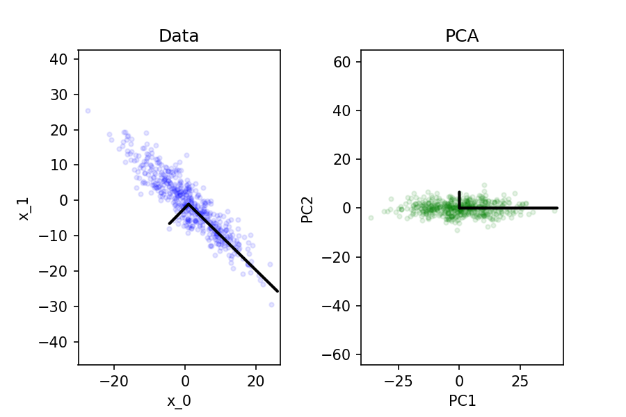
It is easiest to find the first, or "main" axis of the data, and then find subsequent ones. We can also see all the data has been centered -- this ensures our components are not skewed one way or another, and originate from 0.
[4] Finally, to actually solve this, we use Single Value Decomposition (SVD).
SVD
Given an \(\X \in \bb{R}^{n \times d}\), SVD decomposes \(\X\) into the following: \[ \X = \vec{U} \vec{\Sigma} \vec{V}\t \]
- \(\vec{\Sigma} \in \bb{R}^{n \times d} \) is a diagonal matrix of eigenvalues
- \(\vec{U} \in \bb{R}^{n \times n}\) is an orthonormal matrix (orthogonal* and normal columns)
- \(\vec{V}\t \in \bb{R}^{d \times d}\) is our orthogonal matrix of components.
In linear PCA, \(\vec{V}\t = \W\). We can then take the top \(k\) rows.
*a matrix A is orthogonal if \(\vec{A}^{-1} = \vec{A}\t\).
The eigenvalues in \(\vec{\Sigma}\) are related to \(\nm{\X}\t \nm{\X} \) (where \(\nm{\X}\) is the normalised matrix X). The actual eigenvalues are \(\fr{\vec{\Sigma}.^2}{n-1}\) (\(.^2 \) is element wise squared), though I have not found this to be useful.
\(\vec{U}\) is simply not useful. And \(\vec{V}\t \equiv \W\) is very useful.
To approximate on test data, we need our mean \(\vecu{\mu_j}\) from the training data, and our components \(\W\).
Given \(\tilde{\X}\), center it using \(\vecu{\mu_j}\), then compute the new \(\tilde{\Z}\): \[ \tilde{\Z} = \tilde{\X}\W\t \] And we can use \(\Z\). We can work out the reconstruction error by doing \(\lVert \tilde{\Z} \W - \tilde{\X} \rVert_F^2\)
Linear Classification
Linear Classification
Binary Linear Classification
Linear Classification is the idea of using regression models to do classification.
To do binary classification, we need to convert the class to a numerical value that we can compare to -- for positive and negative values of \(y_i\), replace the positive with +1, and the negative with -1.
From our regression value we then determine a class using the sign function -- sign returns +1 if \(y_i > 0\), -1 if \(y_i < 0\), and 0 if \(y_i = 0\). The 0-result is a decision boundary, much like in KNN. We'll just pretend these don't exist for now.

There are many lines which produce the same decision boundary, and so it may be difficult to immediately solve for an answer.
Often, it is better to just draw the decision boundary, and not necessarily the line itself. This also means that we don't need a dimension for y.
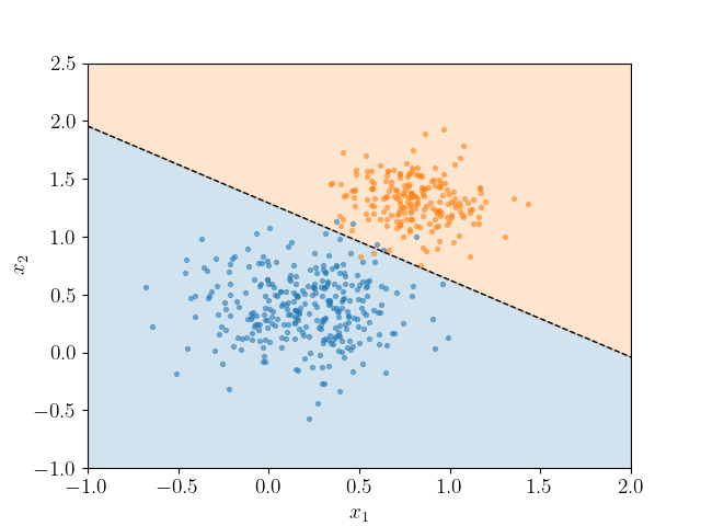
This splits the data into two half-spaces, for the two classes.
If we can split the data into two with that straight line, we say it is linearly separable.
Losses
One simple error to use is the 0-1 Loss -- count the number of wrong predictions. \[ \cal{L}_{0-1}(\ypred, y_i) = \begin{cases} 0 &\rm{if } \ypred = y_i \\ 1 &\rm{if } \ypred \neq y_i \end{cases} \pod{\textrm{ or simply } [\ypred \neq y_i]} \] However, the 0-1 loss is a step function, and has a gradient of 0 everywhere -- rather inconvenient when doing the calculus.
Thus what we want instead is a convex approximation that has the same effect as 0-1 loss:
If \(\w \cdot \x_i > 0 \land y > 0\), this is a correct prediction.
If \(\w \cdot \x_i < 0 \land y < 0 \equiv -\w \cdot \x_i > 0 \land y < 0\), this is a correct prediction.
(Mismatched less than greater thans are incorrect)
Thus doing some rearranging a correct prediction is always if \(y_i \w \cdot x_i > 0\). A wrong prediction should always be 0 to approximate 0-1. However, we are trying to minimise errors, so we reverse everything with a minus:
Thus, we can have a loss function of \[ \cal{L}(\w) = \sum_{i=1}^n \max(0, -y_i\w \cdot \x_i) \]
However, with this loss there is the chance that \(\cal{L}(\w = \vec{0}) = 0\): i.e. absolutely no weights gets 0 loss. In this case, we are not learning, and the solution is degenerate
We change this by adding an offset, s.t. instead of \(y_i \w \cdot \x_i > 0\), do \(y_i \w \cdot \x_i \geq 1\). This is called hinge loss. Whilst this penalises a small section of valid weights, it solves our degeneracy problem. \[ \cal{L}(\w) = \sum_{i=1}^n \max(0, 1-y_i\w \cdot \x_i) \]
Hinge loss is still not smooth, however (it has a fold), and we prefer smooth graphs, so we will "smooth out" the max by using a log-sum-exp method: \(\max(0, y_i \w \cdot \x_i) \approx \log(e^0+ e^{y_i \w \cdot \x_i} \), giving us the most popular loss function: logistic loss.
Logistic Loss is given as \[ \cal{L}(\w) = \sum_{i=1}^n \log(1+ e^{y_i \w \cdot \x_i}) \] and linear classification using this loss has another name: Logicstic Regression [Classifier].

Blue: Hinge loss
Green: Logistic Loss
Confusion Matrix
Multi-class Classification
We can extend logistic regression to multiple classes.
One vs All. for \(k\) possible classes, train \(k\) binary classifiers, based on the two classes \(\in, \not\in\) (in that class or not)
Apply all classifiers to a feature, and return the highest scoring (argmax).
We can even do this in one go - put all the weights of the different classifiers as rows in a matrix \[ \W_{(k \times d)} = \begin{bmatrix} \lla \w_1 \lra \\ \vdots \\ \lla \w_k \lra \end{bmatrix} \] Then just predict all classes \(\hat{\y}_i = \W\t \x_i\), or predict the entire set with \(\hat{\vec{Y}} = \X\W\t\).
Problem: this assumes all classes are independent (they are not).
Softmax Loss. We want to train the model dependently. It is sufficient to have our loss be that the correct class is predicted highest: \[ \w_c \cdot \x_i \geq \max_{\forall k} (\w_{k} \cdot \x_i) \] The value of \(\w \cdot \x_i\) for the correct class \(c\) is the largest value amongst all the possible \(k\) (including \(c\)).
Max is not smooth, and so we do the same log-sum-exp step like logistic: \begin{align} 0 \geq &-\w_c \cdot \x_i + \log(\sum_{k=1}^K \exp(\w_k \cdot \x_i)) \\ \iff &-\log \left(\fr{ \exp{(y_{i}^{correct})} }{ \sum_{k=1}^K \exp(\w_ k \cdot \x_i )}\right) \end{align} Where \(y_{i}^{correct}\) is our \(\w_c \cdot \x_i\) from earlier. This is called softmax loss. From this, we assemble a full loss function, which is commonly called categorical cross-entropy:
Again, I'm using dot product notation, slides consistently use matrix notation \(\w_k\t \x_i\). Just bear this in mind.
Categorical Cross-Entropy, softmax loss with L2-reg, is thus given as \[ \cal{L}(\W) = \sum_{i=1}^n \left( -\w_c \cdot \x_i + \log\left(\sum_{k=1}^K \exp(\w_k \cdot \x_i) \right) \right) + \fr{\lambda}{2} \lVert\W \rVert_F^2 \]
The Perceptron Algorithm
The Perceptron is an alternate representation of a linear classifier, and also the basis to neural networks.

It's graphical; individual features are represented as nodes, and links in the graph represent weights. Features × weights. In this way, it roughly mimics how (biological) neurons work (hence neural networks)
The idea is to find a vector of weights \(\w\) that linearly separate data, same as logistic regression. We iteratively improve the weights over epochs (iterations), with \(\w^0\) being initial wegihts, and \(\w^t\) being the weights at epoch \(t\).
[*] Note: can replace with while there are still errors, but if the data is not linearly separable, this will loop.
[**] Note 2: original material doesn't include learning rate \(\alpha\) -- this means \(\alpha = 1\).
The use of \(y_i \x_i\) has the same idea as logistic loss - because y is -1 or +1. this encourages \(\w\) to tend towards the right prediction for those features \(x_i\) (and discourages tending to the wrong prediction), repeated enough, all the features should "smooth out" and get you a good \(\w\).
Adding a bias is the same as adding an extra input node with a constant value 1.
For multi-class perceptron, because there are multiple classes, you may have to do the encouraging (+) and discouraging (-) separately, because classes will be one-hot encoded.
Support Vector Machines
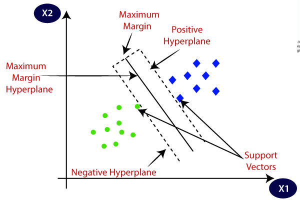

Decision boundary of linear classifier is perpendicular to the line itself. There may be multiple permissible boundaries.
The "best" boundary is one that maximises the difference between nearest points (vectors) -- maximises the margin between them.
The points (vectors) closest to the line, that define the margin, are thus the support vectors.
Optimising. Set the weights such that \(\w \cdot \x_i = +1,\; \w\cdot\x_j = -1\), for the two support vectors \(\x_i, \x_j\) (anything beyond that is more negative, and more positive).
Thus given the distance between the two support vectors is \(d\), we know \(\w \cdot \x_i = 1\) is the same as \(\w \cdot(\x_j + d \fr{\w}{|\w|}) = 1\). Rearranging this we get \[d |\w| = 2 \iff d = \fr{2}{|\w|}\]
Thus maximise \(d = \fr{2}{|\w|}\), which is the same as minimising \(\fr{1}{2}|\w|\), or \(\fr{1}{2}|\w|^2\).
Minimise \(\fr{1}{2}\lVert\w\rVert^2\), subject to
\[ \begin{matrix} \w \cdot \x_i \geq 1 & \rm{for } y_i = 1 \\ \w \cdot \x_i \leq -1 & \rm{for } y_i = -1 \end{matrix} \]The violation is how much "off" they are: for \(y_i = 1, \w \cdot \x_i = -0.5\), the violation is 1.5.
This is just hinge loss - SVMs are L2 regularised hinge loss.
Multiclass SVMs
We want to find a loss that encourages the largest \(\vec{w}_c \cdot \vec{x}_i\) to be the correct prediction, denoted \(\vec{w}_{y_i} \cdot \vec{x}_i\). Definable as $$ \vec{w}_{y_i} \cdot \vec{x}_i > \vec{w}_{c} \cdot \vec{x}_i \pod{\forall c \neq y_i} $$ But penalising violations is "degenerate" (vecs equal to 0), thus can redefine as \begin{align} \vec{w}_{y_i} \cdot \vec{x}_i &\geq \vec{w}_{c} \cdot \vec{x}_i +1\pod{\forall c \neq y_i}\\ \implies 0 &\geq 1 - \vec{w}_{y_i} \cdot \vec{x}_i +\vec{w}_{c}\cdot \vec{x}_i \end{align}
Two ways to measure violation:
- The sum of all violations: $$ \sum\limits_{c \neq y_i} \max(0, 1 - \vec{w}_{y_i} \cdot \vec{x}_i +\vec{w}_{c}\cdot \vec{x}_i) \longrightarrow SUM $$
- The largest violation: $$ \max_{c \neq y_i}(\max(0, 1 - \vec{w}_{y_i} \cdot \vec{x}_i +\vec{w}_{c}\cdot \vec{x}_i)) \longrightarrow MAX $$
This gives us a loss function of $$ \begin{matrix}\mathcal{L}(\vec{W}) = \sum\limits_{i=1}^n SUM + \frac{\lambda}{2}||\vec{W}||^2_F& \textrm{or}& \mathcal{L}(\vec{W}) = \sum\limits_{i=1}^n MAX\end{matrix} + \frac{\lambda}{2}||\vec{W}||_F^2 $$
For \(k\) classes,
- SUM gives a penalty of \(k-1\) for \(\vec{w}_c = 0\)
- MAX gives a penalty of 1 instead.
Kernel Trick
Sometimes, your data is not linearly separable. But it is separable if you re-basis it, such as polynomial regression:
- By converting features from \(\X = \begin{bmatrix} \x_1& \x_2 \end{bmatrix}\) to \(\Z = \begin{bmatrix} 1 & \x_1 & \x_2 & (\x_1)^2 & (\x_2)^2 & \x_1 \x_2 \end{bmatrix}\) we are separating with polynomials.
- But note that we go from 2d to 6d, if we want to correctly do it, and this becomes a problem with high dimensions.
We can merge L2 regularisation into our prediction formula, and get an equation \[ \vec{v} = \Z\t (\Z \Z\t + \lambda \vec{I})^{-1} \y \] for a new set of weights \(\vec{v}\) based on our new basis.
- L2 Reg: \[\cal{L}(\vec{v}) = \fr{1}{2} \lVert \Z\vec{v} - \y \rVert^2 + \fr{\lambda}{2} \lVert \vec{v} \rVert\]
- \[ \nabla \cal{L}(\vec{v}) = \Z\t\Z \vec{v} - \Z\t \y + \lambda\vec{v} \]
- \[ \implies \vec{v} = (\Z\t \Z + \lambda \vec{I})^{-1} (\Z\t \y) \] where \(Z_{(k \times k)}\) is always invertible
- \[ \implies \vec{v} = \left[ \Z\t (\Z \Z\t + \lambda \vec{I})^{-1} \right]_{(n \times n)} \y \]
Now for test data \(\tl{\X}\) predict \(\hat{\y}\) by computing \(\tl{\Z}\): \begin{align} \hat{\y} &= \tl{\Z} \vec{v} \\ &= \tl{\Z} \Z\t (\Z \Z\t + \lambda \vec{I})^{-1} \y \end{align}
This is however computationaly expensive, but we have the blocks \(\tl{\Z} \Z\t,\; \Z\Z\t\), and so let us call them \(\tl{\vec{K}}, \vec{K}\).
The \(\vec{K}\) is now the kernel matrix, and is an \(n \times n\) matrix computed from \(\Z\). Each cell \(k_{ij}\) is just \(\z_i \cdot \z_j\).
The kernel trick is to simply not: don't calculate \(\Z\), calculate \(\vec{K}\) directly
Example. Let \(\x_i = (a, b), \; \x_j = (c, d)\).
To do quadratics, we can: get \(\z_i = (a^2, ab\sqrt{2}, b^2)\) and \(\z_j = (c^2, cd\sqrt{2}, d^2)\)
The dot product \(\z_i \cdot \z_j =\) \begin{align} &= a^2 c^2 + (ab\sqrt{2} )(cd\sqrt{2}) + b^2 d^2 \\ &= (ac + bd)^2 \\ &= (\x_i \cdot \x_j) ^2 \end{align}
i.e. there's no point to \(\z\), just have a kernel function \(\kappa(\x_i, \x_j) = (\x_i \cdot x_j)^2\) and skip the \(\z\).
We have a kernel function \(\kappa(\x_i, \x_j)\) that computes cell \(k_{ij}\) of the kernel, skipping the middleman.
They're usually given to us. The kernel function must obey Mercer's Theorem.
Theorem. Rather than first mapping from X to Z with a function \(\phi : \X \lra \Z\), we instead compute a modified inner product \(\kappa(a, \b) = \phi(a) \cdot \phi(b)\), which is a function that fits a bunch of formal stuff, but most importantly is symmetric: \(\kappa(a, b) = \kappa(b,a)\)
Now, the process becomes
- Form \(\vec{K}\) from \(\X\), compute \(\vec{u} = (\vec{K} + \lambda \vec{I}) ^{-1} \y\) (u are weights)
- Form \(\tl{\vec{K}}\) from \(\tl{\X}\), and compute \(\hat{\y} = \tl{\vec{K}} \vec{u}\).
Kernel trick can be extended to non vector data (like text, images), and can be used for multiple things, including PCA.
MLE and MAP estimation
Maximum likelihood / Maximum a-posteriori estimation
Okay, look, I don't *actually* have much of a clue what's going on here.
To clarify notation:
- \(\max(\cdot)\) and \(\min(\cdot)\) return the maximum and minimum value of a function, w.r.t a parameter.
- \(\argmax(\cdot)\) returns the *parameter* that achieves the maximum (or minimum) value
- In some case, argmin, argmax return sets: $$ \begin{align*} \argmin_w((w-1)^2) &\equiv \{1\}\\ \argmax_w(\cos w) &\equiv \{\dots, -2\pi, 0, 2\pi, \dots\} \end{align*} $$
MLE
Assume a dataset D with parameter \(w\). Ex. flip a coin 3 times and get HHT, parameter \(w\) is the likelihood that the probability lands on heads.
The likelihood of D is a probability mass function \(p(D|w)\): prob of observing D given parameter \(w\)
- Given \(D = \{H,T,T\}\) and \(w=0.5\), then \(p(D|w) = 0.5 \times 0.5 \times 0.5 = 0.125\)
- Given \(w=0\) then \(p(D|w) = 0\).
You can plot \(p(D=\{\cdots\}|w)\) w.r.t. D and \(w\). If this is continous, you have a probability distribution. Since it's w.r.t D, the area under the dist does not sum to 1.
We get the maximum likelihood estimation: \[ MLE = \hat{w} \in \argmax_{w}(p(D|w)) \]
To compute MLE, we can use argmin, and minimise the negative-log-likelihood: \[ \argmax_\vec{w} (p(D|\vec{w})) \equiv \argmin_\vec{w}(-\log(p(D|\vec{w}))) \] We want to switch it to minimise so we can integrate it as a normal log function, also log removes multiplications which makes things more efficient: \[ \log(\alpha\beta) = \log\alpha + \log\beta \]
If our dataset D has \(n\) examples: \[ p(D|\vec{w}) = \prod_{i=1}^n p(\vec{x}_i | \vec{w}) \] Then MLE would be \[ \vec{\hat{w}} \in \argmax_\vec{w} (p(D|\vec{w})) \equiv \argmin_\vec{w}(-\sum\limits_{i=1}^n \log p(\vec{x_i}|\vec{w})) \]
Least Squares is Gaussian MLE. Recall least squares: minimise errors squared. If we grab the errors \(\epsilon_i\) and plot a histogram of error occurences, it forms a gaussian (normal) dist.
More generally, have \(y_i = \vec{w}\cdot \vec{x_i} + \epsilon_i\) where \(\epsilon_i\) follows a normal dist, \[ p(\epsilon_i) = \frac{1}{\sqrt{2\pi}}\exp(-\frac{\epsilon_i^2}{2}) \] we have a gaussian likelihood for \(y_i\): \[ p(y_i|\vec{x_i},\vec{w}) = \frac{1}{\sqrt{2\pi}}\exp\left(-\frac{(\vec{w}\cdot\vec{x_i}-y_i)^2}{2}\right)\longrightarrow G(\vec{w, \vec{x_i}}) \] Then we just find \(\argmin_\vec{w}(-\sum\limits_{i=1}^n \log(G(\vec{x_i,w})))\).
After simplifying, the inner function of the argmin leads to \(-\sum\limits \left[\log\frac{1}{\sqrt{2\pi}} - \frac{1}{2}(\vec{w} \cdot \vec{x_i} - y_i)^2 \right]\) (\(\log\exp\) cancels.)
Thus finally, we get a \(k + \frac{1}{2}\sum\limits_{i=1}^n (\vec{w}\cdot \vec{x_i}-y_i)^2\) for some constant \(k\), and to minimise this, is just to minimise least squares.
Example. MLE for a normal dist. Assume that samples \(\vec{X} = \{\vec{x_i}\dots \vec{x_n}\}\) and their conditional probability is normal dist: \[ p(\vec{X}|\mu, \sigma) = \left(\frac{1}{\sigma \sqrt{2\pi}}\right)^n \exp\left( -\frac{1}{2\sigma^2} \sum\limits_{i=1}^n(\vec{x_i} - \mu^2) \right) \] We want to find the MLE \[ \hat{\mu}, \hat{\sigma} \in \argmin(-\log(p)) \] Which is a quadratic function. To find the minima, we can compute partial derivatives w.r.t \(\mu, \sigma\).
Solving for \(\mu,\sigma\), we can get \[ \begin{align*} \hat{\mu} &= \frac{1}{n}\sum\limits_{i=1}^n \vec{x_i} \\ \hat{\sigma^2} &= \frac{1}{n}\sum\limits_{i=1}^n (\vec{\hat{x}_i} - \hat{\mu})^2 \end{align*} \]
Recommender Systems
Neural Networks
Contents
Neural Networks

One of these is **sigmoid**: $$ h(x) = \fr{1}{1 + e^{-x}} $$ Which maps $x \longrightarrow [0, 1]$
An activation function that may be used for \(y_i\), for classification could be the **step** function: $$ h(x) = \begin{cases} 1 & x > 0 \\ -1 & x < 0 \end{cases} $$
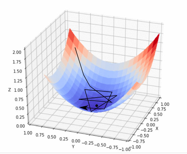
NNs are trained with **stochastic gradient descent**. For one hidden layer, an MSE loss is given as $$ \cal{L}(\W, \v) = \fr{1}{n} \sum_{i=1}^n (\v\t h(\W\t \x_i) - y_i)^2 $$ The gradient of a random sample is calculated, and is propagated back through the network and incrementally update weights -- **backpropagation**. Rather than using one sample, we can take a random subset of samples, a **minibatch**. $$ \w^{t+1} = \w^t - \alpha^t \fr{1}{|B^t|} \sum_{i \in B^t} \left(\nabla \cal{L}_i (\w^t) \right) $$ The challenging region of SGD is *inversely proportional* to batch size. Note on terminology: * **Epoch**: a full pass through the training set. * **Iteration**: a single SGD update (i.e. batch number)
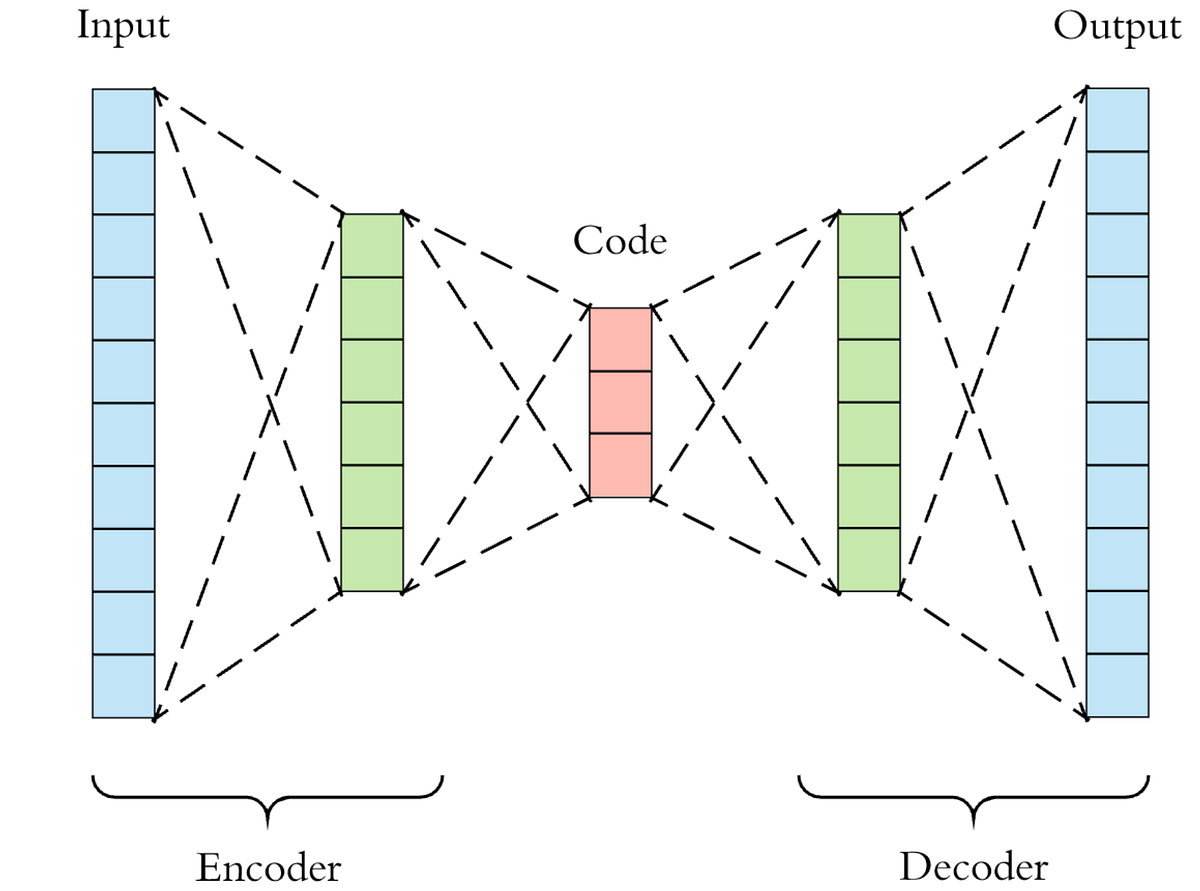
Autoencoders
Ensemble Methods

So far, we've been talking about majority vote. Other ensemble methods include * Averaging * Stacking * Bagging / Bootstrap * Random forest * Boosting / cascading
***Averaging.*** Technically, majority vote is a type of averaging, for classification ensemble models. For regression ensemble methods we can take the mean instead. If classifiers are overfit, we can still consider that they are overfit in different ways and thus mitigate the effect.
***Stacking.*** Using a separate, different classfier to compile together the results of your ensemble.

#### Bias-Variance Decomposition ***Bagging.*** The general idea is to train the same type of classifier **several times** over **different subsets** of the training data. i.e. you get a set of models over the same source, but different training data. This reduces the **variance** in expected error.


***Random Forest.*** (actually one of my favourite models before I did this damn module) Bagged decision trees, but also: * When defining a node, only use a small proportion (e.g. $\sqrt{d}$) of the total $d$ features to split on. So whilst a particular tree may overfit, the overall will be much more independent. It happens to be one of the best "black box" no-tuning ML algorithms.
And
