Introduction
Contents
- Rational Agents
- Uninformed Search
- Informed Search
- Constraint Satisfaction Problems
- Local Search
- Adversarial Search
- Knowledge Representation
- Planning with Certainty
- Planning with Uncertainty
Introduction to Artificial Intelligence
A defintion of artificial intelligence can fall under 4 categories:
| Thinking humanly | Thinking rationally |
| Thinking rationally | Acting rationally |
Acting Humanly
The Turing Test is a well known test for how well an AI performs. It suggests that if it is acting intelligently, it is thinking intelligently.
It also suggests that an AI requires knowledge, reasoning, learning (and language).
However the general consensus is that the Turing Test is not great, as many counterexamples and exploits can be found for it.
One such "counterexample" is Searle's Chinese Room.
Thinking Humanly
There is a field of study called cognitive modelling, which is modelling human thinking in programs. (We will however ignore this)
Thinking rationally
Given a premise/some premises, an agent (the AI model) must derive or deduce the solution via logic. Rational deduction however has problems dealing with uncertainty.
Acting Rationally
Acting rationally can be summed up as "doing the right thing", which is to say, the action that maximises some achievement metric. However, thought or inference in these actions is not necessarily involved.
In actuality, the boundaries between these four categories are quite blurred.
Specialised AI vs AGI
Rational Agents
Specifically, we look at Rational Agents.
These agents can be modelled as a function \(f:P \longrightarrow A\), where P denotes percept histories and A denotes actions.
Agents are typically required to exhibit autonomy, and seek the best performance possible. (Perfect rationality may not always be the best as there is a trade off with computing resources)
Rational Agents
Introduction
Agent Input Model

Above shows a diagram of what inputs an agent takes, and what it does.
Rational Agents
The Goals of a rational agent can be specified by a performance measure, which is a numerical value.
A rational action is an action which aims to maximise the performance measure, given the percept history to date.
Note that an agent is not onmiscient, clairvoyant (forseeing changes), nor always successful. The expected value, not the actual value, is considered - an action to maximise expected value which fails is still rational.
Dimensions of Complexity
Dimensions of Complexity
The design space / considerations of an AI can be defined by a set of "dimensions of complexity".
| Dimension | Values |
|---|---|
| Modularity | Flat, modular, heirarchical |
| Planning Horizon | Static/none, finite (stage), indefinite, infinite |
| Representation | Flat state, features, relations |
| Computational Limits | Perfect or bounded rationality |
| Learning | Knowledge given or learned |
| Sensing Uncertainty | Fully or partially obervable |
| Effect Uncertainty | Deterministic, stochastic |
| Preference | Goals, complex preferences |
| Number of Agents | Single, multiple |
| Interaction | Offline, online |
Modularity
Modularity concerns the structure and abstraction.
- Flat where the agent only has 1 level of abstraction
- Modular where the agent has interacting modules that can be separately understood
- Hierarchical where the agent has modules that (recursively) decompose into others
Planning Horizon
Planning Horizon concerns how the world is, and how far forward does the agent plan to.
- Static, where the world does not change
- Finite Stage, where the agent reasons for a fixed number of timesteps
- Indefinite State, agent reasons about a finite, not predetermined number of steps
- Infinite Stage, agent plans for going forever (process oriented)
Representation
Finding compact Representations and exploiting them for computational gains. An AI can reason in
- Explicit States, where a state describes everything about a world
- Features/Propositions, which are descriptors of states. A few features can lead to a lot of states.
- Individuals and their relations, a feature for each relationship on each tuple of individuals. Thus an agent can reason without knowing the individuals or if there are infinite individuals.
Computational Limits
Computational Limits:
- Perfect rationality is ideal, but does not take into account computing resources
- Bounded rationality is what we hope to achieve, good descisions made accounting for perceptual and computing limitations
Learning from Experience
Learning from Experience:
- Where knowledge is given
- Or knowledge is learned from data or past experience
Uncertainty
Uncertainty has two dimensions: sensing and effect. In each, an agent can have:
- No (uncertainty), agent knows what is true
- Disjunctive, a set of states are possible
- Probabilistic, there is a probability distribution between states
Sensing Uncertainty
Sensing Uncertainty is about what the agent can sense about state, the state can be
- Fully observable
- Partially observable (possible number of states from obs.)
Effect Uncertainty
Effect Uncertainty concerns whether an agent could predict an outcome from a state and an action.
- Deterministic environments say yes
- Stochastic environments say no (have uncertainty).
Preferences
Preferences concerns what an agent tries to achieve.
- Achievement goal is a single goal to achieve - can be a (complex) logical formula
- Complex preferences involve tradeoffs between various desires, with priorities. These are further split into Ordinal (order priority matters) and Cardinal (specific absolute values also matter).
Number of Agents
Crucially, Number of reasoning agents.
- Single Agent reasoning relegates every other agent as environment and not really considered, whilst
- Multiple Agent reasoning involves an agent reasoning strategically about other agents.
Interaction
Interaction talks about when the agent reasons relating to its action
- Reason offline, before acting
- Reason online, whilst interacting with environment
Examples
Some examples of the dimensions of different agents
| Dimension | Values |
|---|---|
| Modularity | Flat |
| Planning Horizon | indefinite |
| Representation | Flat state |
| Computational Limits | Perfect rationality |
| Learning | Knowledge given |
| Sensing Uncertainty | Fully obervable |
| Effect Uncertainty | Deterministic |
| Preference | Goals |
| Number of Agents | Single |
| Interaction | Offline |
| Dimension | Values |
|---|---|
| Modularity | Flat |
| Planning Horizon | indefinite, infinite |
| Representation | features |
| Computational Limits | Perfect rationality |
| Learning | Knowledge learned |
| Sensing Uncertainty | Fully obervable |
| Effect Uncertainty | Stochastic |
| Preference | complex preferences |
| Number of Agents | Single |
| Interaction | online |
| Dimension | Values |
|---|---|
| Modularity | heirarchical |
| Planning Horizon | indefinite, infinite |
| Representation | relations |
| Computational Limits | bounded rationality |
| Learning | Knowledge learned |
| Sensing Uncertainty | partially obervable |
| Effect Uncertainty | stochastic |
| Preference | complex preferences |
| Number of Agents | multiple |
| Interaction | online |
Complex interaction
Dimensions intract and combine in complex ways. Partial observability makes multi-agent and indefinite stage more complex, and with modularity you can have fully or partially observcable modules. Heirarchical reasoning, Individuals and relations, and bounded rationality make reasoning simpler.
Representations and Solutions
Representations

A task can be represented in a formal way, from which we can make formal deductions and interpret them to get our solution.
We want a representation complex enough to solve the problem, to be as close to the problem as possible, but also compact, natural, and maintainable.
We want it to be amenable to computation, thus
(1) Can express features which can be exploited for computational gain
(1) Can tradeoff between accuracy and time/space complexity
And able to acquire data from people, datasets, and past experiences.
Defining a Solution
Given informal description of problem, what is the solution? Much is usually unspecified, but they cannot be arbitrarily filled.
Much work in AI is for common-sense reasoning, the agent needs to make common sense deductions about unstated assumptions.
Quality of Solutions
Solutions can be split into classes of quality
- Optimal solution: the best solution (for the quality measure)
- Satisficing solution: a good-enough solution (that meets good-enough criteria)
- Approximately optimal solution: close but not quite to best in theory
- Probable solution: unproved, but likely to be good enough
Descisions and Outcomes
Good descisions can have bad outcomes (and vice versa). Information can lead to better descisions, known as value of information.
We can often tradeoff computation time and complexity: an anytime algorithm can provide a solution at any time, but more time can lead to better answer.
An agent is also concerned with acquiring appropriate information, timely computation, besides finding the right answer.
We can often use a quality over time graph with a time discount to represent this.

Choosing a Representation
Problem \(\longrightarrow\) specificiation of problem \(\longrightarrow\) appropriate computation.
We need to choose a representation, this can be done as a high level formal/natural specificaiton, down to programming languages, assembly, etc, etc.
Physical Symbol Hypothesis
We define a Symbol as a meaninigful physical pattern that can be manipulated (like logic symbols)
A Symbol system creates, copies, modifies, and deletes symbols.
The Physical symbol hypothesis states that a physical symb. system is necessary and sufficient for general intelligent action
Knowledge and Symbol Levels
Two levels of abstraction common amongst systems:
- The knowledge level, what an agent knows, its goals.
- The symbol level, a description of agent in terms of its reasoning (internal symbolic reasoning).
Mapping problem to representation
We have a few questions to ask
- What level of abstraction to use?
- What individuals and relations to represent?
- How can knowledge be represented s.t. natural, modular, and maintainable?
- How can agent acquire information from data, sensing, experience, etc?
Choosing Level of Abstraction
A high level description is easier for human understanding. A lower level abstraction however can be more accurate, predictive, however are harder to reason, specify, understand. One may not know all details for a low level description. Many cases lead to multipe levels of abstraction.
Reasoning and Acting
Reasoning is computation required to determine what action to do.
- Design time reasoning is where computation is done by designer beforehand. Offline and Online, similar to the complex dimension, is either deciding before starting to act (using knowledge from the knowledge base) or deciding between receiving information and acting respectively.
Uninformed Search
Introduction
Problem Solving
Problem Solving
Often we are only given the specification for a solution, and have to search for it. A typical situation is where we have an agent in one state, and have a set of deterministic actions with which it will go towards the goal state.
Often this can be abstrated into finding the goal state in a directed graph of linked states.
Example
Suppose you're in Coventry and want to get to London. How do you achieve this?
Using what transport do you get there? What routes do you go via? More importantly, which routes are reasonable?
Finding the actions that would get you from Coventry to London is problem solving.
A problem-solving agent is a goal-based agent that will determine sequences of actions leading to desirable states. It must in this process determine which states are reasonable to go through.
Problem solving steps
There are 4 steps:
- Goal formulation: identify goal given current situation.
- Problem formulation: Identify permissible actions (operators) and states to consider
- Search: Find the sequence of actions to achieve a goal
- Execution: Perform the actions in the solution
For our example from earlier:
- Formulate goal: be in London
- Formulate problem:
- states: (in which) towns and cities
- operators: drive between towns and cities
- Search: sequence of towns and cities
- Execution: drive
Pseudocode agent
We can make a mockup of an offline reasoning agent in pseudocode.
Naturally all the functions mentioned are left as an excersise to the reader (i.e. assumed implemented).
formulateGoal internally will use its current perceptions.
Problem types
Problems of course can come in many types.
- Single state problem: deterministic and fully observable. Sensors tell agent current state, it knows exactly what to do, can work out what state it will be in after.
- Multiple state problem: deterministic and partially observable. Agent knows its actions, but has limited access to state. There may be a set of states the agent would end up in, agent must manipulate sets.
- Contingency problem: stochastic and partially observable. Agent does not know current state so is unsure of result of action. Must use sensors during execution. Solution is a tree with contingency branches. Search and execution is often interleaved.
- Exploration problem: unknown state space. Agent does not know what it's actions will do, and has to explore and learn. This is an online problem.
Vacuum Cleaner World
Let's use an example of a simple environment, a vacuum robot V and a world with two locations, [ ][ ]. Each location may also contain dirt ([ d] or [Vd] for vacuum and dirt). The vacuum can move left or right, and suck dirt.
Single state. Suppose we know we are in the state [V][d]. We then know our sequence of actions is just [right, suck].
Multiple State. (sensorless / conformant) Suppose we don't know which state we start in. We could have the states:
1. [Vd][ d] |
2. [ d][Vd] |
3. [Vd][ ] |
4. [ d][V ] |
5. [V ][ d] |
6. [ ][Vd] |
7. [V ][ ] |
8. [ ][V ] |
Contingency. Suppose we start in state [V ][ d], but our vacuum has received a downgrade: if we suck a clean square, there is a chance that it may make that square less clean. So what do we do?
What we can is sense whilst acting, thus: [right, if dirt then suck].
State space problems
A State space problem consists of a set of states; subsets of start states, goal states; a set of actions; an action function (f(state, action) -> new state); and a criterion that specifies the quality of an acceptable solution (depends on problem).
Since the real world is complex, state space may require abstraction for problem solving. States, operators, and solutions approximate the real world equivalent, though one must take care that their operations are still valid for the real world counterpart.
8-puzzle
A 3\(\times\)3 grid of tiles numbered 1 to 8, with a blank space for sliding. We want to get from some initial state to some goal state.
283   123
164   8_4
7_5 765- States can be coordinate locations of tiles
- Operators - we want the fewest possible - are moving the blank square up, down, left, or right
- Our goal test would be the given goal state
- The path cost we can set as 1 per operation
State Space Graphs
A general formultion for a problem is a state space graph. It is:
- A directed graph consisting of a set N of nodes, set A of arcs/edges, which are ordered pairs of nodes.
- Node \(n_2\) neighbours node \(n_1\) if there is an arc \(\langle n_1, n_2 \rangle\) (denoted with triangle brackets)
- A path is a sequence of nodes \(\langle n_0, n_1, \cdots, n_k\rangle\) s.t. \(\langle n_{i-1}, n_i \rangle \in A\) (arcs between all nodes)
- The length of a path from \(n_0\) to \(n_k\) is \(k\).
- Given a set of start nodes and goal nodes, a solution is a path from a start node to a goal node.
Tree Searching
Tree searching algorithms
A tree search is a basic approach to problem solving. It is an offline, simulated exploration of the state space. Starting with a start state, we expand an explored state by generating / exploring its successor branches, to build a search tree.
We have a single start state, and repeatedly expand until we find a solution, or run out of valid candidates.
Implementation details
A state represents a physical configuration of a puzzle, and a node will be the data structure for one state of the tree.
A node stores the state, parent, children, depth, path cost - the last of these is usually denoted \(g\).

Nodes (explored) but not yet expanded are called the frontier, and is generally represented as a queue.
Search strategies
The strategy of searching is defined by which order we expand nodes in. These strategies are evaluated over several criteria:
- completeness: will the strategy always find a solution, if it exists?
- optimality: will the best (least cost) solution be found?
- time complexity: The number of nodes expanded - this depends on the maximum branching factor \(b\), depth of best solution \(d\), and the maximum depth of the state space \(m\), which may be \(\infty\).
- space complexity, the maximum number of nodes stored in memory (also in terms of \(b, d, m\))
Simple, uninformed strategies
Uninformed search only uses information given in problem definiton - we have no measure of which nodes would be better to expand to, nor do we really check the nodes once we've explored them (i.e. not checking cycles).
Two of these algorithms are Breadth-first search BFS and Depth-first search DFS.
Breadth first
BFS expands the shallowest node: put recently expanded successors at the end of queue: FIFO.
- Completeness. BFS is complete because it will always find a solution, provided \(b\) finite.
- Time. Since at every node we expand \(b\) branches, in total for a depth of \(d\) we will be expanding \(1 + b + b^2 + b^3 + \cdots + b^d = O(b^d)\) times. This becomes \(O(b^{d+1})\) if the check for goal state is done when that node is about to be expanded, instead of as part of expansion.
- Space. Each leaf node is kept in memory, thus there are \(O(b^{d-1})\) explored nodes and \(O(b^{d})\) in the frontier, and overall space is dominated by frontier, \(O(b^d)\).
- Optimality. BFS is optimal only if the cost function does not decrease.
The main problem for BFS is the space usage, which can balloon very very quickly (with \(b = 10\) and 1 KB per node, at depth 8 one needs around 1 TB of memory).
Depth first
DFS expands the deepest node: put most recently expanded successors at the start of the "queue" (stack): LIFO.
- Completeness. DFS is not complete because it will fail in infinite depth and loop situations. If we avoid repeated paths and have or limit to a finite depth, then DFS is complete.
- Time. \(O(b^m)\), which is O(horrible) if \(m > d\) significantly. Otherwise may be significantly faster than BFS.
- Space. \(O(bm)\), i.e. linear space: store path from root to leaf and unexpanded siblings of nodes on path.
- Optimality. Not guaranteed.
Graph Searching
Notes
This section is uninformed search, and graph searches are similarly uninformed, so much so that the algorithms presented do not even check for cycles, despite common intuition.
The main difference is that in graph search we look at paths, rather than nodes. Expanding into a node would be adding it to the stored path.
Graphs
With trees, if we have looped states these will just branch out to infinity. Graphs are a good way to take loops into account and are a practical representation of such spaces.
Similar to a tree, we incrementally explore, maintaining a frontier of explored paths. The frontier should expand into unexplored nodes until a goal node is encountered.
The way nodes are selected is the search strategy, the neighbours of (all) nodes define a graph, and the goal defines the solution.
We can continue searching from the return call even if a solution has been found, if we want more or all possible solutions.
BFS on Graphs
All paths on the frontier \([p_1 .. p_r]\) are expanded one by one, and the neighbours of an explored path are added to the end of the frontier.
The time complexity is instead written \(O(b^n)\), where \(n\) is the path length (instead of tree depth).
DFS on Graphs
DFS treats the frontier as a stack instead. The time complexity is \(O(b^k)\) where \(k\) is the maximum number of arcs a path can have (i.e. max depth). Space complexity is linear: \(O(k + (b-1))\).
Now, DFS is said to fail on both infinitely long graphs and graphs with cycles, although I'm not sure why you're adding already explored nodes to the frontier (cycle case).
Lowest cost first
Sometimes, there are costs, or weights, associated with edges. The cost of a path is thus the sum of the cost of edges, and an optimal solution has the path with the smallest total cost.
Lowest cost first is a fairly naive algorithm that simply selects the path on the frontier with the lowest cost. I.e., frontier paths are stored in a priority queue according to path length.
Lowest cost is complete.
Supposedly none of these algorithms will halt on a finite graph with cycles, but one has to be a particular type of person to program a graph search without cycle checking / not adding explored nodes to the unexplored frontier.
Informed Search
Introduction
Overview
Uninformed search is inefficient, especially when we have extra information we can exploit. By using problem-specific knowledge, we can improve our searching - this is informed search.
Still offline.
Heuristic Search
Overview
If you know where the goal is, when selecting paths do not ignore it.
Employ the use of an extra heuristic measurement \(h(n)\) - an estimate of the remaining cost to the goal.
This heuristic should be efficient to compute, and always be an underestimate (no path to goal strictly less than \(h(n)\)). If a heuristic meets these criteria, then it is admissible.
Examples
If one is on a euclidean plane finding the shortest path, \(h(n)\) can be the straight-line distance to the goal. If the cost is time, \(h(n)\) can be straight-line distance divided by max speed.
We can think of this as reducing the constraints in the problem to an easier representation that we can quickly calculate an answer for. The straight-line distance does not count obstacles, for example.
Best First Search
When we choose nodes to expand in a frontier, the heuristic can determine the order / rank of the frontier structure.
Heuristic DFS is where we select a neighbour such that the best neighbour is selected first.
If by best we mean closest (by some metric) distance to the goal, then we have Greedy Best First Search (BFS).
The frontier is a priority queue ordered by \(h(n)\).
Problems
Some graphs are very much not good for BFS. Especially if we do not track cycles.

Analysis
BFS has an exponential space complexity, of \(O(b^n\) where \(b\) is the branching factor and \(n\) is the number of nodes. TIme complexity is also \(O(b^n)\).
It is not guaranteed to find the solution, even if one exists, and may not necessarily find the shortest path (but will go in its general direction).
A* Search
A* Search
A* considers both path cost and heuristic values. We denote the cost of a path \(p\) by \(g(p)\) or \(cost(p)\), and the estimate of remaining path to goal is \(h(p)\).
Let \(f(p) = cost(p) + h(p)\), at some node on the path \(p\). \(f(p)\) is thus the overall estimate cost of \(p\). A* searches using this estimate value.
Thus A* can be considered as a mix of lowest-cost and best-first, and its frontier is a priority queue ordered by the metric \(f\).
Admissibility
A* is admissible if
- The branching factor is finite
- Arc costs are bounded above some positive number (cannot just be \(>0\) because we'd get Zeno's Paradox )
- \(h(n)\) is non-negative and an underestimate
Justification. A path \(p\) is selected by A*. Suppose another path \(p'\) ends on the frontier. Since \(p\) is chosen before \(p'\), by definition \[cost(p) \leq cost(p') + h(p')\] And since \(h\) is an underestimate \(cost(p') + h(p') \leq cost(p'_C)\), where \(p'_C\) is a complete path extending \(p'\) and reaching the goal. By definition of the algorithm, we must have for any other unpicked path \(p'_C\) \[cost(p) \leq cost(p'_C).\]
A* can always find a solution if there is one.
The frontier always contains part of a path to the goal, and A* will halt as the costs of the paths increase beyond any finite number.
However, this doesn't mean A* won't pick unoptimal nodes, just that its final result is always the optiumal path (even if we have cycles in our graph).
Heuristics are not equal
Some heuristics are better than others. The closer a heuristic is to the true value (without overestimating), the more efficient A* is.
For some optimal cost \(c\), A* will explore all paths \(p:cost(p) + h(p) < c\). A* will explore some paths \(q:cost(q) + h(q) = c\) (until it finds the solution), and will not explore overestimates.
Thus the closer the underestimate, the less paths there are where \(cost(p) + h(p) < c\). Additionally, if the number of paths where \(cost(p) + h(p) = c\) is large, then there may be much variability in space and time of A*.
Complexity
A* is exponential time in \(h\)-error \(\times\) path length to solution. A* is also exponential space, since it stores all nodes in memory.
Pruning, Cycle Checking, and Restrictions
Cycle Checking
Before, we have not dealt with the cases where a search algorithm hits an already visited node (i.e. go in a cycle). If this is so, we can "prune" a path that leads into a cycle, removing all unnecessary nodes from consideration.
In depth-first methods, cycle checking can be done in \(O(1)\) with things like hash functions. In most other algoirthms though this is often \(O(n)\).
Multiple Path Pruning
Similarly, this pruning can apply when we have two paths to the same node. We can prune the path to said node and keep just the existing path.
THis can be implemented via a set of explored nodes at the end of explored paths, the closed list.
When a path \(\langle n_0 \cdots n_k \rangle\) is selected, if \(n_k \in\) closed list, then discard path, otherwise add \(n_k\) to list and proceed on.
On optimal solutions
How do we make sure we do not prune a path whcih is better than the already found one?
The most straightforward answer is to make sure that you always select the best path first, though this may be hard. We could remove all paths which use the longer route, but those paths may extend further (past the node which the better route reaches), and that's a lot of work wasted.
Otherwise we can simply replace the longer path: given a path \(p = \langle s \cdots n \cdots m \rangle\) if \(p' = \langle s \cdots n \rangle\) is found which is shorter than the corresponding part in \(p\), replace that specific segment.
Path Pruning and A*
A* selects a path \(p'\) to node \(n'\). Suppose there's a shorter path to \(n'\), via a path \(p\), which currently ends at the fronter node \(n\) (so \(len(p') > len(p) + len(\langle n \cdots n' \rangle )\)).
Since \(p'\) was selected before \(p\), \(f(p') \leq f(p)\), thus \(cost(p') + h(p') \leq cost(p) + h(p)\). Let \(cost(n, n')\) be the real length of a path \(\langle n \cdots n' \rangle\). Since \(p\) is lower cost than \(p'\), \(cost(p) + cost(n, n') < cost(p')\). \begin{align} \implies cost(p') - cost(p) &\leq h(p) - h(p') \\ \textrm{and } cost(n, n') & < cost(p') - cost(p) \\ h(p) - h(p') &= h(n) - h(n') \\ \implies cost(n, n') & < h(n) - h(n') \end{align} If we make sure \(|h(n) - h(n')| \leq cost(n, n')\) then this situation will never happen (always select the best path first option).
Monotone Restriction
A heuristic \(h\) satisfies monotone restriction if \(|h(m) - h(n)| \leq cost(m, n) \; \forall \textrm{arcs } \langle m, n \rangle\). It is then termed consistent.
A* with a consistent heuristic and path pruning always finds the shortest path.
Changing Directions
Direction of Search
In graph/tree searches, the direction we search doesn't really matter. We can go from goal to start nodes.
Whilst the forward branching factor is the number of arcs out of a node, the backwards branching factor is the number of arcs going into a node.
If the forward factor is larger than backwards factor, our \(O(b^n)\) algorithm would do much better searching backwards.
Of course, a backwards graph isn't always available.
Bidirectional Search
We have a \(O(b^k)\) (\(k\) depth of goal) algorithm. We can get it to be less horrible by searching from both sides simultaneously. \(2b^{\frac{k}{2}} < b^k\) after all.
The main problem with this is making sure both sides meet.
Oftentimes, BFS is used from the goal for a full set of locations that leads to goal, whilst another method is used from the start to link up the path.
Island Hopping
An island driven search is like an extension of the bidirectional search - we have a series of "islands": useful nodes that can link a start and a finish, \[s \longrightarrow i_1 \longrightarrow i_2 \longrightarrow \cdots \longrightarrow i_m \longrightarrow t\] Now, we have \(m\) subproblems to solve, which can improve efficiency to \(mb^{\frac{k}{m}} \).
The difficult is then in identifying the correct islands, and it's hard to guarantee optimality with such an approach.
Dynamic Programming
Dynamic programming is a fancy way of saying have an array of values you update and retrieve from as you go along. This is explained more in depth in CS260.
We build a table \(D: D_n = \) the distance of shortest path from \(n\) to the goal. Then, apply the following strategy: \[D_n = \begin{cases} &0 &\textrm{if isGoal}(n) \\ &\min_{\forall \langle m, n \rangle} (|\langle m, n \rangle| + D_m) &\textrm{otherwise}\end{cases}\]
Bounded DFS
A bounded DFS does normal DFS, but has a cost/depth bound at which it will stop exploring. Only part of the search graph is explored.
We do this because DFS uses linear space and if space is tight it's appropriate.
Iterative Deepening
If we bounded-DFS over an ever increasing bound, we have iterative deepening. Starting with a bound \(b = 0\), do DFS, and either return the solution or increase the bound.
This finds the first solution BFS does, but uses linear space. There is an overhead of \(\frac{b}{b-1} \times\) the cost of expanding a node at depth \(k\) with BFS; i.e. bounded DFS will do \(\frac{b}{b-1} \times\) more work than DFS at the same \(b\) depth. As \(b\) increases, overhead decreases.
Depth-First Branch & Bound
Depth first branch and bound Combines DFS with heuristic info, and so will find an optimal solution. More useful if multiple solutions, and still has the space complexity of DFS.
We want to find a single optimal solution. Suppose \(b\) is the cost of the shortest path to goal so far.
What if we then encounter a path \(p : cost(p) + h(p) \geq b\)? \(p\) can be pruned. If we instead communicate a path \(q : q\) is better, then \(q\)'s cost can be \(b\) and the path \(q\) remembered.
This is linear space (since DFS) and we can guarantee an optimal solution when it completes.
Initalising Bound
We can initialise the bound \(b\) to \(\infty\). We can also set it to an estimate of the minimum path cost.
After DFS terminates, either (1) a solution found, (2) no solution found, no path pruned, (3) no solution found, path pruned.
Can be combined with iterative deepening to increase the bound until a solution is found.
Cycle pruning works well, but multiple path pruning does not, since storing extra paths defeats the point of saving space with DFS.
Admissible Heuristics
The 8-puzzle example
The branching factor is roughly 3, and a typical solution is 20 steps. Thus, an exhaustive search is \(3^20\) states, and there are \(9!\) non-repeating states. It would be nice to have a heuristic to search with.
We could:
- \(h_1(n)\) the number of misplaced tiles - admissible since each misplaced tile must be moved at least once
- \(h_2(n)\) the Manhattan (city block) distance of each tile - admissible since a single move can only move one step orthogonally.
Characterising Heuristics
Definition. If A* search expands \(N\) nodes and solution is depth \(d\), then the effective branching factor \(b* \) is the factor a uniform tree of depth \(d\) must have to have \(N\) nodes. \[N = 1 + b* + (b*)^2 + \dots + (b*)^d\] Ex. depth 5 and 52 nodes: \(b* = 1.91\).
As \(b* \longrightarrow 1\), the larger the problem that can be solved (efficiently).
Whilst solving for \(b* \) may be difficult, we can estimate it experimentally, over small instances.
On the prior example, an experiment determined that \(h_2\) is better than \(h_1\) (lower EBF).
Definition. If some \(h_2(n) \geq h_1(n) \; \forall n\) then \(h_2\) dominates \(h_1\).
Note that whilst an (admissible) heuristic which is closer to the true cost is better, we must make sure the heuristic still remains cheap to calculate.
Deriving Heuristics - Relaxed problems
Admissible heuristics can be the exact solutions of problems with certain conditions relaxed.
If the problem is defined in formal language this is easier.
We may generate several different relaxed problems, and thus may have several admissible heuristics. If one dominates, use that. Else, if you have \(h_1, h_2, \dots, h_n\) admissible heuristics which do not dominate each other, just use \(h = \max(h_1, h_2, \dots, h_n)\).
Because all options are admissible, the aggregate \(h\) is admissible - and dominates each constituent individually.
Example
If we describe the 8-puzzle as "A tile can move from square A to B if A is adjacent to B, and B is blank", then we can generate some relaxed problems:
- A tile can move from A to B if A adjacent to B
- A tile can move from A to B if B is blank
- A tile can move from A to B
Subproblems
We can derive a heuristic from a subproblem.
For the 8 puzzle, we can only solve the problem for 4 squares (ignoring 5-8), and use that as a heuristic. Of course, the subproblem should be pretty easy to solve.
Pattern Databases
We can then store the possible solution costs for each instance of a subproblem in a data structure for easy lookup. Then the heuristic is the looked-up cost of the corresponding subproblem.
Different pattern databases can also be combined to get a maximum of them all.
Disjoint Pattern Databases
If we have multiple independent subproblems, we can store them in different databases and add them together.
These databases form disjoint pattern databases.
Other approaches
We can run searches over smaller training problems, and use the statistical results as a heuristic.
Say we have a base heuristic \(\eta\). If in 95% our training sets, \(\eta = 14\) when the real cost is 18, we can just use \(h = 18\) as our statistical heuristic.
Now this is not admissible, but can often be quite efficient (and good enough).
Constraint Satisfaction Problems
Contents
- Varialbes, Constraints, and Worlds
- Constraint Satisfaction
- Consistency Algorithms
- Domain Splitting
- Variable Elimination
Variables, Constraints, and Worlds
Varibles
Constraint Satisfaction Problems (CSPs) are described with regards to variables and configurations of variables (worlds).
Algebraic Variables are symbols used to describe features. Often denoted with capital letters, like \(X\), which have a corresponding domain of possible values, \(D_X\) or \(dom(X)\).
Symbols internally are just labels - they only have meaning to the user. The meaning associated to a variable should follow the clarity principle, that an omniscient agent can determine values knowing meaning of the variables.
Discrete Variables has a finite or countably infinite domain - a special type of discrete variable with domain size 2 is a binary variable, most often seen as boolean variables.
Continuous Variables have uncountably infinite domain, e.g. \(\mathbb{R}\)
Assignments and Worlds
Given a set of variables, an assignment is a function \(: \textrm{vars} \rightarrow \textrm{dom(vars)}\). Variables \(\{X_1, X_2, \dots, X_n\} \) would have an assignment \(\{X_1 = v_1, X_2 = v_2, \dots, X_n = v_n\} : v_i \in D_{X_i} \).
A total assignment assigns all variables, since assignments can be partial.
A possible world is a total assignment. If \(X_i\) has value \(v_i\) in the assignment of a world \(w\), then we say "variable \(X_i\) has value \(v_i\) in world \(w\).
The number of worlds is product of all domains: \(|W| = \prod^n_{i=1} |D_{X_i}|\)
The advantage of using variables over pure discrete states is that a few variables can describe many states.
Constraints
A (hard) constraint specificies legal combinations of some variables.
A scope is a set of (relevant) variables, a constraint \(C\) is just a relation on that scopt \(C : S \longrightarrow \{T, F\}\), which involves each variable in scope.
An assignment \(A\) on the full set of variables \(S'\) (i.e. the superset of the scope / \(S \subseteq S'\)) satisfies a constraint on \(S\) if everything maps to true. Else, the constraint is violated.
Constraints can be defined by intension and extension. Intension is "define by rule", where formulae are used. Extension is "define by enumeration", where the valid combinations are listed out.
A unary constraint is on 1 variable, a binary on two, etc.
Constraint Satisfaction
CSPs
A CSP consists of a set of variables, a domain per variable, and a set of constraints. The goal is to make true (satisfy) all constraints.
A finite CSP has a finite set of variables, with finite domains. We will usually be dealing with these. Note that some algorithms which work for one type of CSP may not work for others.
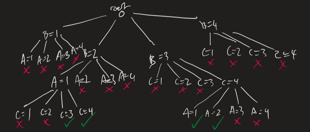
Example. A delivery robot must carry out activities \(a,b,c,d,e\). Those activities happen at any time 1, 2, 3, 4. Let \(A\) be variable of activity \(a\). The domains of all variables are thus \(\{1,2,3,4\}\). The following must be satisfied: \[\{ B \neq 3, C \neq 2, A \neq B, B \neq C, C < D, A = D, E < A, E < B, E < C, E < D, B \neq D\} \]
When we have a CSP, a number of tasks are helpful for it:
- Determine if there is a solution
- Find the solution model
- Count the number of models / enumerate them
- Find the best model (given some metric)
- Determine if some assertion holds
Generate and Test
Obviously the simplest way to solve a CSP is via a generate-and-test (G&T) algorithm - to solve via exhaustion.
Let \(D\) be the "assignment space" (set of total assignments), G&T will generate a random assignment, and save it.
Complexity
G&T is an \(O(\textrm{horrible})\) algorithm.
For \(n\) variables each with domain size \(d\), and \(e\) constraints, the total number of constraints tested is \(O(ed^n)\). It's fine for small problems but can quickly spiral out of control.
G&T assigns values to all variables regardless, but some constraints are unary, so some values can be ruled out even before generating.
Backtracking Search
Backtracking is about tree-searching a tree constructed from incremental assignments of variables in a CSP.
We define the search space as thus:
- Nodes are assignments of values
- Neighbours of a node \(n\) are gotten by selecting some var \(Y \neq n\) and assigning a value, then checking constraints
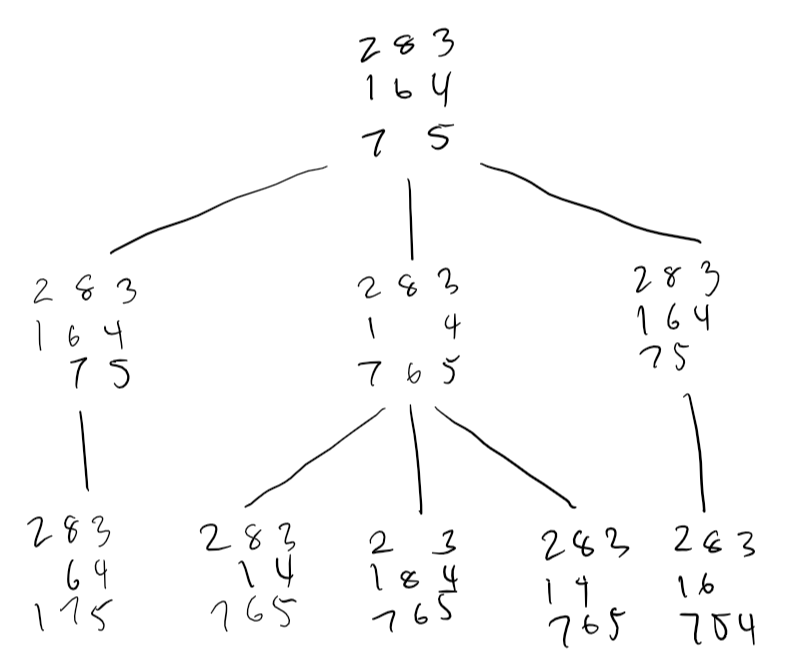
Example. Let us have a CSP with variables \(A, B, C\) each with domain \(\{1,2,3,4\} \), with constraints \((A < B), (B < C)\). A search tree can be drawn:
Since all goals are at depth \(n\) (\(n\) vars), we use DFS to save space. The branching factor \(b = (n-l)d\) for a depth \(l\) and domain size \(d\).
Implementation
We can implement backtracking as the following:
Selection heuristic
How do we select a variable? How do we assign a value? We use heuristics (which can be combined) to determine which to select.
- MRV · Minimum Remaining Values: select the variable with fewest possible values.
- Most Degrees: variable with the most constraints - often used as a tiebreaker to MRV.
- LCV · Least Constraining Value: assign a value which rules out the least other values.
Consistency Algorithms
Introduction
Though DFS is an improvement on G&T, it still isn't that good.
In example 2, the DFS searched through all possible alignments in a domain, even if they were clearly contradictory with one or more other variables.
We could interleave an algorithm that removes all impossible values given the current assigned domains and the constraints.
Consistency Algorithms
Consistency algorithms operate on a network of constraints:
Each node is a variable, which is annotated with its domain. Each arc between nodes is a constraint over those variables, and annotated with the rule of said constraint.
We say that for a variable \(X\), \(D_X\) will now be the set of possible values (which initially is its domain). For every constraint \(c,\; \forall X\) in scope of \( c ,\; \exists \textrm{ arc } \langle X, c \rangle\).
Another way is to represent variables as round nodes and constraints as rectangular ones, with an arc between a varaible and a constraint meaning that variable is in scope of that constraint.
Arc Consistency
In the simplest case, the constraint is unary. The variable is then domain consistent if all values satisfy the constraint.
Then, let constraint \(c\) have the scope \(\{X_1, Y_1, \dots, Y_k\} \). Arc \(\langle X, c \rangle\) is arc consistent if \(\forall x \in D_x\), \(\exists y_1 \dots y_k : y_i \in D_{Y_i} : c(X=x, Y_1=y_1, \dots, Y_k = y_k)\) is satisfied. I.e. every value for X has some compatible assignments for all other variables.
A network is arc consistent if all arcs are consistent.
If an arc is not consistent, then \(\exists x \in D_X\) which is incompatible with some other variables in the constraint. We can delete values to make an arc consistent.
Though deleting a value from one \(D_X\), it may make other constraint arcs with \(X\) inconsistent again, so these need to be redone. We compile all of this into an algorithm like so:
Algorithm Description
- GAC keeps track of a (toDo) list of unconsidered arcs, which are initially all arcs in the graph.
- Until the to do list is expended, we pick and remove an arc every time, and making it consistent with regards to the constraint (\(c\)). If we make any changes, this may adversely affect all other constraints including (X).
- Thus, for all other constraints (\(c'\)), we need to add the arcs for all other variables in those constraints (\(Z \neq X\)) to the to do list to reconsider again.
Regardless of arc selection order, the algorithm will terminate with the same arc-consistent graph and set of domains. Three cases will happen:
- A domain becomes \(\varnothing \implies\) no solution to CSP
- Each domain has 1 value \(\implies\) unique solution
- All or some domains have multiple values \(\implies\) we do not know the solution and will have to use another method to find it
Note Well: Arc consistent algorithms can still have no solutions. Example: Take a CSP with variables \(A, B, C\) all with domain \(\{1,2,3\} \), and constraints \(A = B, B = C, C \neq A\). The graph is arc consistent - but as we can clearly see there are no possible solutions.
Complexity
Assume we have only binary constraints.
Suppose there are \(c\) many constraints, and the domain of each variable is size \(d\). There are thus \(2c\) arcs. Checking the arc \(\langle X, c = r(X, Y) \rangle\)* is at the worst case iterating through each domain value in \(Y\) for each in \(X\), thus making \(O(d^2)\).
*As mentioned previously \(c\) is a relation, \(c = r(X,Y)\) is just denoting that it's over the variables X and Y.
The arc may need to be checked once for each element in \(dom(Y)\), which is \(O(cd)\).
Thus time complexity of GAC on binary constraints is order \(O(cd^3)\), which is linear on \(c\).
The space complexity of GAC is \(O(nd)\) for \(n\) variables.
Extensions
The domain need not be finite - and many be specified through intensions.
If constraints defined extensionally, when we prune a value from X, we can prune that value from all other constraints including X.
Higher order techniques like path consistency can consider \(k\)-tuples of vars at once - this may deal with the "arc consistent but no solution" problem but is often less efficient.
Domain Splitting
Splitting domains
Another method of simplifying a network is to split a problem into disjoint cases, then unioning together the solutions.
We can split a problem into several disjoint subproblems through splitting the domain of a variable, having multiple "worlds" in a sense where the variable is assigned different things.
Suppose \(X : D_X = \{T, F\} \). We can find solutions for where \(X = T\) and \(X = F\) separately.
The idea is that this reduces the problem into smaller subproblems which are easier and faster to solve. Also, if we just want any solution, we can look in one subproblem, and only if no solution we move onto the other.
We have multiple strategies of splitting if the domain is larger than 2. For \(X:D_X = \{1,2,3,4\} \), we could either split into 4 "worlds" of \(X=1,2,3,4\) respectively, or 2 "worlds" where \(X=\{1,2\} \) and \(X = \{3,4\} \), for example. The former makes more progress per split, whilst the latter can do more pruning with fewer steps.
Note that recursively splitting domains into units (and recognising impossible configurations) is literally how the backtrack search works.
Interleaving
It is more efficient to interleave arc consistency with searching/splitting. We can alternate between arc consistency, and domain splitting.
Implementation
Extensions
It is possible to find all solutions, by altering such that \(\varnothing\) is returned when no solution found, and a set union of all solutions otherwise.
If assigning a variable disconnects the graph (that variable connects two separate components), then the soluion is just the cross product of the two components - this shortcut saves computation when counting components.
Variable Elimination
Problem Structure
We can break a CSP of \(n\) variables up into separate subproblems of \(c\) variables each.
Each solving step takes \(O(d^c)\) (domain size \(d\)), so in total we have \(O(\frac{n}{c}d^c)\), which, through a bit of trickery, is actually linear in \(n\).
But this is genuinely much better: take \(n=80, d=2, c=20\). The whole problem takes \(O(d^n) = 2^{80}\) which is 4 billion years at 10 million processes a second. Splitting it using \(c=20\) we get \(4 \times 2^{20}\) which is 0.4 seconds at same speed.
Tree structures and conditioning
A CSP graph without loops can be solved in \(O(nd^2)\), with the following algorithm:
- Choose a variable as root, and order from root to leaves such that all nodes' parents preceeds them in ordering
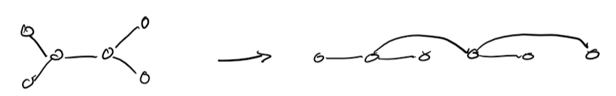
- for (j = 1 .. n), make (x_j) consistent with its parents
However, most of the time we don't have a tree, but removing one or two variables would make it a tree.
Conditioning is the process of instantiating (assigning) a variable and proving compatibility with neighbours such that the rest of the graph resolves down into a tree.
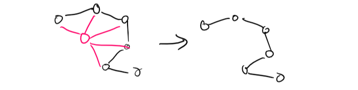
Cutset Conditioning is conditioning but done to a set of variables (a cutset).
Variable Elimination
More generally we can look at simplifying a CSP by "removing" variables from consideration.
When we remove a variable X, we need to ensure that we preserve the effect of X in all remaining constraints, so we can get back from reduced form to the original problem.
The idea is to collect all constraints involving X, (natural) join all the constraints to make \(c_x(X, \bar{Y})\) where \(\bar{Y} \) is all other variables neighbouring X. Then, project onto (select columns of) \(\bar{Y} \) only, and this one big relation would then replace all relations including X.
Natural join is denoted \(\bowtie\), can see CS258 / SQL natural join for how it works.
Say we have a table \(r\) with \(A, B, C\), the projection onto \(B, C\) is denoted \(\pi_{\{B, C\}}r\), with \(\pi\) standing for project - it's akin to select distinct from B, C.
Example. Let us have a CSP with variables \(A, B, C\) each with domains \(\{1,2,3,4\}\). We want to remove B. The constraints involving B are \(A < B\) and \(B < C\).
\[ \begin{bmatrix} A & B \\ 1 & 2 \\ 1 & 3 \\ 1 & 4 \\ 2 & 3 \\ 2 & 4 \\ 3 & 4 \end{bmatrix} \bowtie \begin{bmatrix} B & C \\ 1 & 2 \\ 1 & 3 \\ 1 & 4 \\ 2 & 3 \\ 2 & 4 \\ 3 & 4 \end{bmatrix} = \begin{bmatrix} A & B & C \\ 1 & 2 & 3 \\ 1 & 2 & 4 \\ 1 & 3 & 4 \\ 2 & 3 & 4 \end{bmatrix} \]
To get the "induced" relation on A and C (removing B), we project the relation table (call it \(r\)) onto A and B: \[ \pi_{\{A, C\}}r = \begin{bmatrix} A & C \\ 1 & 3 \\ 1 & 4 \\ 2 & 4 \end{bmatrix} \]
The original constraints are replaced by this one on A and C. The original constraint however is remembered to reconstruct the full problem afterwards.
Implementation
We can implement this recursively:
Efficiency
Efficiency depends on how \(X\) is selected. The intermediate structure depends only on the graph of the constraint network.
Variable Elimination is only effective if the network is sparse.
The Treewidth is the number of variables in the largest relation. The graph treewidth is the minimum treewidth of any ordering.
VE is exponential in treewidth, and linear in variables, whereas searching is exponential in variables.
Heuristic
We have some heurisics to detrmine what variable to eliminate.
- Min-factor: select var which results in smallest relation
- Min-deficiency select var which adds the fewest arcs to the remaining network. The deficiency of a variable \(X = \) number of pairs in the relation with \(X\) that are not in a relation with each other -- "It is ok to remove a variable and create a large relation if it doesn't make the network more complicated"
Local Search
Contents
Iterative Improvement
Local Search
In some problems, only the goal state is important, whilst the path to it is not.
Local search is an approach which only cares about the current state, and surrounding states it can move to.
Whilst local search is not systematic, it is efficient for memory and can often find reasonable solutions, and is useful for many optimisation problems, where there is some objective cost/"goodness" function.
We define the state space as all possible configurations (states) of a world, and the goal as the state we want to end up in. Usually this is optimal by some heuristic metric.
Iterative Improvement Algorithms
Iterative improvements describe algorithms that only consider the current state, and all states it can move to. The idea is to move to a state which gives the greatest increase in "quality" (metric based)
Since we only track current state, these algorithms are usually constant space (though time is eugheheheh?).
Common Problems
One common problem in computer science is called the N-Queens Problem, where, given an \(n \times n\) chessboard, fit \(n\) queens on it so that none can take another in one move.
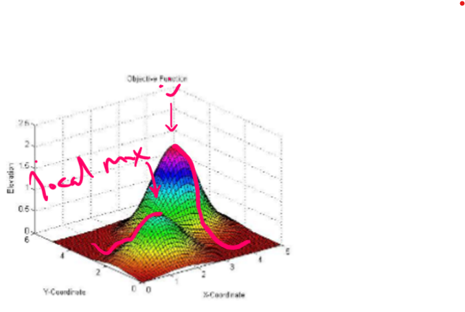
Another, more general problem, is an abstraction of many problems. Imagine you have two values for a state, and a cost metric. The highest optimal costs form "peaks" in a landscape, and the goal is to travel to the highest possible peak.
Hill Climbing
Hill Climbing, or Greedy Local Search, is the most basic of iterative improvement algorithms, and always tries to improve state (by reducing or increasing a cost function depending on the situation).
There is no search tree, and if there are several equally good values, they are chosen at random.
Implementation
Problems
Local maxima: naive hill climbing is very supceptible to finding local maxima: states that are surrounded by worse states, but not being the best state overall in the state space. Thus, the algorithm will halt sub-optimally. We will talk about ways to solve this later.
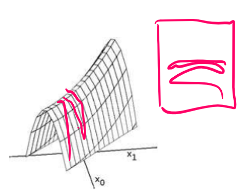
Ridges: whilst not as big of a problem, if we have a ridge with very steep sides, the search algorithm may oscillate around the ridge, thus making very slow uphill progress.
Plateaus: A large flat expanse will cause a random walk. This may be a local maximum plateau, or a "shoulder plateau" (where one edge leads to higher ground, whilst the others lower). We need to allow sidways motion to try get off a plateau if it's a shoulder, but this must be limited, else we would walk infinitely.
Greedy descent for CSPs
Greedy Descent is a hill climbing algorithm for CSPs.
The idea is to maintain an assignment of variables to values (initialised randomly). Select a variable to change, and select a new value for said variable, repeat until a satisfying arrangement is found.
When we assign values randomly to variables, we can break constraints. Each broken constraint is one conflict, and our goal is to get an assignment with zero conflicts. So we can use the number of conflicts as our heuristic measurement.
Selecting variables
We want to find the variable-value pair that minimises the number of conflicts. There are multiple strategies to select:
- Select variable that participates in most conflicts, and a value that minimises those conflicts
- Select a variable that appears in any conflict, and a value that minimises that number
- Select a variable at random and (same as above)
- Select a variable and value at random, and accept if it doesn't increase the number of conflicts
More Complex Domains
When domains are small / unordered, the neighbours of one state can be equivalent to choosing another value for a variable. When domains are large / ordered, the neighbours can be considered as adjacent values.
If the domains are continuous (imagine a function) we use a process called gradient descent, which changes a variable proportional to its heuristic (cost) function. i.e. We find the gradient at that point (via differentiation), and then go in the opposite direction by a certain step size \(\eta\), to "descend" down to minimise cost. \[X_i : v_i \longrightarrow v_i - \eta \frac{\partial h}{\partial X_i}\] Which is saying, variable \(X_i\) goes from value \(v_i\) to a value one gradient step away (the \(\del\) thing is the derivative).
Stochasticity
Randomised Greedy Descent
Stochasticity is a fancy word for randomness. The idea in general is to introduce some randomness into our choices, so we don't beeline it for the local maxima, and gives the algorithm a chance to find the actual maximum.
There are two main methods of randomising greedy descent. Random Steps, where we sometimes move to a random neighbour instead of the best one, and Random restart, where we start again somewhere else, and take the best out of all runs.
If the space has jagged, small local minima, then random steps can take us closer to the true minima, but random restart alone would get start. Conversely, if the space is wide with tall peaks, random restart can be quite quick, but random steps wouldn't get out of a minima well at all.
Stochastic Local Search
Stochastic local search is greedy descent with a mix of both random steps and random restart.
Randomly Walking
When doing a search step, have a fixed percentage where you choose another variable (or value).
Perhaps choose the variable that is in most conficts, perhaps choose any in-conflict variable, or just any variable altogether.
Sometimes choose the best value, but sometimes choose a random value instead.
Comparing Stochastic Algorithms
Stochastic algorithms are inherently random, and so how do we measure how good they are? It depends on how much time you have, and how reliable the algorithm is at halting.
You run tests on three algorithms, A, B, and C. A is very quick (say, 0.4s) at solving 30% of a problem set, but doesn't halt for the other 70%. B is 60% at reasonable speed (1m), but doesn't halt for anything else, and C is 100% of problems, but takes ages (like 20m) for each one.
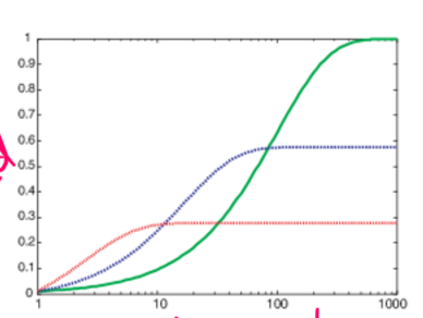
By plotting a graph like shown, we can then determine which algorithm is best for our needs. If our problem is solution critical, then we would go for C, since it always finds a solution. If we need time critical, then A, ran multiple times (with a 30% chance of success each time) might be more preferable.
Variants on Stochastic Algorithms
Simulated Annealing
Annealing is a process in metallurgy that heat-treats a metal to change its properties. We take the vague concepts from this example and apply it to a CSP by "heat treating" the variables.
We have a temperature parameter, \(T\), which slowly decreases over time.
Now, we pick a variable, and a value at random. If it is an improvement, we always adopt it. If it's not better, with probability based on \(T\), we adopt it anyway.
Note: the actual probability is based on the heuristic \(h()\) of the two values. If we have a current value of \(n\) and a new value of \(n'\), the probability we adopt it is \( e^{\frac{h(n')-h(n)}{T}} \).
And as we do more iterations, this probablity \(T\) goes down, representing us "honing in" on a target.
"Tabu" Lists
Sometimes our search space has cycles, and we do not want that. A Tabu List (not "taboo"?) is a list of the last \(k\) explored states, that we do not allow moving into.
This is like keeping track of all states, but much less memory and work intensive (depending on the size of \(k\)).
Parallel Search
Similar to random restart, a parallel search does the same thing ... but in parallel. One total assignment is called an individual, and we have \(k\) individuals, all run at once, all updated every step, and get the solutions of all those \(k\) searches.
The first solution to return (i.e. the quickest), or the best solution out of all solved, is taken as the final solution. You could probably multithread this.
Beam Search
A beam search is like parallel search, where we have a number of individuals. Every update, however, instead of each individual picking one best neighbour, they pick \(k\) best neighbours, which then pick \(k\) best neighbours, and so on.
When \(k = 1\), we have greedy descent, and when \(k = \infty\), we have breadth-first search. Being able to pick \(k\) allows us to limit the amount of space and parallelism we use.
Stochastic Beam Search
Expanding on from beam search, a stochastic beam search picks not the best \(k\) individuals, but rather \(k\) individuals based on probability weighted by their heuristic scores (best heuristics are more likely to be picked).
This maintains diversity and allows some beams to find different local maxima / the global maxima. We can think of this as akin to asexual reproduction.
Genetic Algorithms
A Generic Algoritm (GA) is a self-improvement algorithm based off Darwin's theory of evolution (and is kinda like AI Eugenics). It is often used for training neural networks, but can also be used for CSPs.
We have a population of \(k\) randomly generated individuals (states). Each individual is represented as a string describing the state, to facilitate computation.
Successor states are generated based on two "parent" states, like sexual reproduction.
Individuals can be evaluated by a fitness function, which should return higher values for better states. The fitness of an individual is related to the probability that individual is allowed to "reproduce". All individuals not chosen / below the threshold are culled (discarded)
"Reproduction"
For each chosen pair from a GA, a random "crossover point" is chosen. Two offspring are generated by swapping the parent strings after the crossover point.
Parents "123|41234" and "567|85678", and a crossover point of 3 (shown in parent), generate the children "12385678" and "56741234".
Finally, each children is subject to a random mutation with a small probability, changing maybe one letter.
Please note an individual can be chosen more than once to reproduce (though obviously not with itself)
Running style
If parents are quite different, their children will be quite different from both parents.
Thus a GA takes very large steps at the beginning, and slow down as the population begins to converge around some optimal states. This is useful for optimisation problems.
The choice of represenation is fundamental - a representation needs to be a meaningful description for a GA to work properly.
Adversarial Search
Introduction
Adversarial Search
Consider a multi-agent environment, where agents are in direct conflict with each other. These type of games give rise to adversarial search.
Opponents to an agent creates uncertainty, which the agent must deal with by considering contingencies.
These games are often complex, and time is usually important and limited, thus the agent may have to "best guess" based on experience and what it can calculate to be the best in the time allowed.
Uncertainty may not only arise from opponent moves, but also from other factors, like randomness of dice, or time being limited as to not allow perfect decision making.
This uncertainty makes games interesting, and a better representation of the real world.
- A decision must be made even if optimal cannot be made
- Inefficiency is penalised - a slow program loses!
Perfect Decisions
Let's first consider games which are small enough that we can make a perfect decision.
Games, formally
For a given game, we have:
- An initial state which we start in
- A set of operators or "successor functions" - this defines all legal moves and their resulting states
- A terminal test, which determines if the agent is in a terminal state, i.e. when the game is over
- A utility function (aka payoff function), which assigns a numerical value to terminal states describing how good they are - +1 win, 0 draw, -1 lose for example.
Noughts and Crosses
Let's consider the game Noughts and Crosses. It's sufficiently small and simple that we can build a tree for it.
In the game we can win, draw or lose. These terminal states can be given the utility 1, 0, -1 respectively.
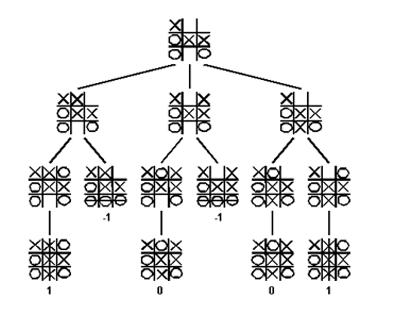
Let's call our players Min and Max. Max goes first, and Min goes second. When points are awarded, if Max wins the points are positive, and if Max loses, the points are negative.
Max wants to maximise the score, Min wants to minimise it, and so every turn after Max plays, Min will try to prevent Max from winning and getting positive score. Max thus needs a strategy to prevent Min from stopping him, or worse, winning.
Obviously as Max we don't know what Min will do, so we have to plan for every possible move Min can do.
Perfect decisions
If we have such a formal, deterministic game (such as noughts and crosses, draughts, chess, etc), we can consider perfect decisions: making the best decision considering every eventuality.
Course for some games (like chess) there are too many options to realistically consider, perfect decision making is not practical, but a computer could perfectly play noughts and crosses.
Two ply game trees
Let's step back and consider a generic two player game. Each move of the game is when all players have played, and since there are two players, the game tree is called two-ply.
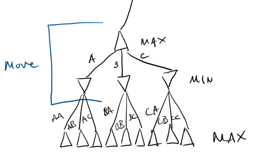
We denote Max's moves with an up arrow \(\Delta\), and Min's moves with a down arrow \(\nabla\), as their names would suggest.
Max has three of nine possible moves to make against Min, depending on what move Min makes. When we represent a game as a tree like this, we can use this to make an algorithm for an optimal move for Max.
Minimax
Assuming both players are perfectly rational players, minimax is an algorithm that gives the optimal strategy for Max.
Given a state of the game, pick the move that has the largest minimax value — describing the best possible outcome for Max against the best possible opponent: \[ \textrm{minimaxValue}(n) = \begin{cases} \textrm{utility}(n) & n \textrm{ is a terminal state} \\ \max_{s \in \textrm{successor}(n)}(\textrm{minimaxValue}(s)) & n \textrm{ is a node for Max} \\ \min_{s \in \textrm{successor}(n)}(\textrm{minimaxValue}(s)) & n \textrm{ is a node for Min} \end{cases} \]
Process
- Generate a complete game tree
- Use the utility function to value the terminal states
- Use these values to assign values to one level up
- Repeat until the root state
- Pick node with highest utility from the children
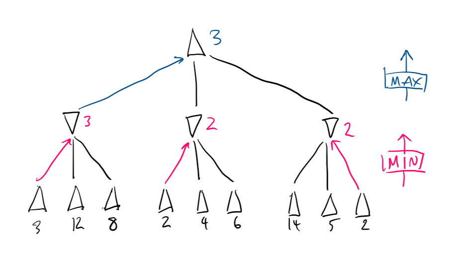
Min nodes are rated using the lowest of its children (magenta)
Max nodes are rated using the highest of its children (blue)
Max picks the left move.
Completeness
Minimax is complete ... should the tree be finite. It is also optimal ... given your opponent is too.
Minimax takes \(O(bd)\) (b branching, d depth) since it is DFS and requires \(O(b^d)\), which is really \(O(\textrm{horrible})\) for complex games.
This is because minimax requires a complete search tree, which, if you have too many combinations, is a no-go.
Multiplayer Minimax!?
Instead of storing utility as a single value, we can store a vector for every player playing. Thus, we can minimax for three or more-ply games.
Then, with some math magic relevant to the game structure, we can max everyone for their own utility against everyone else.
Alpha-Beta Pruning
Overview
\(\alpha \beta\)-pruning is based on minimax, and gets its name from the utilities on the min-max tree.
- \(\alpha\) is the best choice along the path for Max
- \(\beta\) is the best choice along the path for Min
The pruning part comes from when we search through the search tree. In short, if we discover a node which makes a path objectively worse than any other already found, we don't bother to search more on that path, and prune it out entirely - terminate the recursive call.
Example. Take the game state shown earlier.
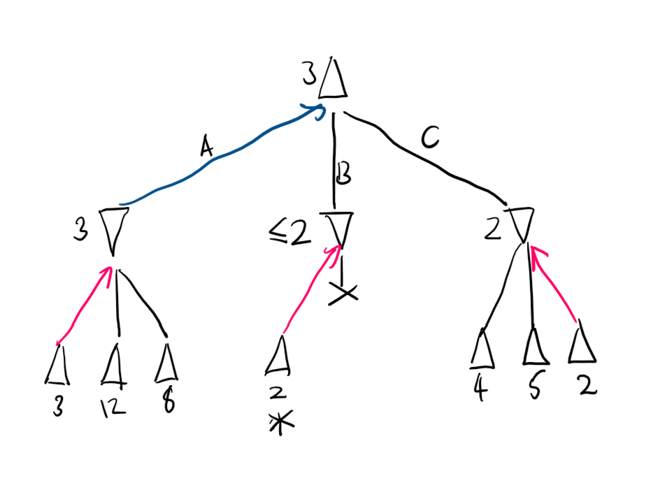
We run minimax from left to right, so the A path is searched for Max. We find that the value we get is 3.
The B path is searched, and we immediately come across a terminal node with value 2. Since Min will always try to minimise score, it will never pick anything above 2 for that branch, thus A will always be better. We stop searching B and prune it.
Finally, we search C. The 2 value is only found in the last child, and so everything is searched anyway.
Finally, Max plays A.
Effectiveness
The effectiveness of ab-pruning depends on the order we search in. For example above, the second branch was pruned very quicky but the third was fully searched.
To fix this we could examine the best successors first, reducing minimax from \(O(b^d)\) to \(O(b^{\frac{d}{2 }})\) - a significant improvement.
Looking at successors randomly is roughly \(O(b^{\frac{3}{4}d})\), which is still better than nothing.
In practice, always looking at the best successor is very difficult, but even a simple ordering function gives a significant speedup. A ✨heuristic✨ of sorts.
Games with Chance
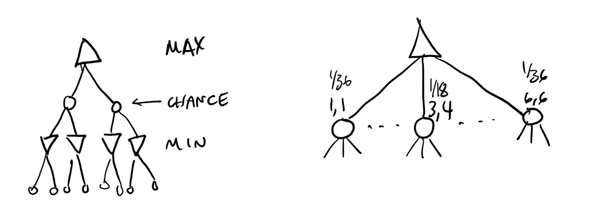
Chance nodes
So far we have only looked at perfectly deterministic games - those where the only "uncertainty" comes from opponent moves.
However, a lot of games contain elements of chance, moves being dependent on the roll of a dice.
We thus have to include chance nodes, labelled with the value, and the chance of obtaining that value. We can then calculate an expected value talking into account the probabilities.
Expected minimiax
We can expand the minimax value function further by taking into account expected values: \[ \textrm{expMinMax}(n) = \begin{cases} \textrm{utility}(n) & n \textrm{ is terminal node} \\ \max_{s \in \textrm{successor}(n)}(\textrm{expMinMax}(s)) & n \textrm{ is node for Max} \\ \min_{s \in \textrm{successor}(n)}(\textrm{expMinMax}(s)) & n \textrm{ is node for Min} \\ \sum_{s \in \textrm{successor}(n)}(P(s) \cdot \textrm{expMinMax}(s)) & n \textrm{ is chance node} \end{cases} \] Since this considers all outcomes, it has a big O of horrible at \(O(b^m n^m)\) where \(n\) is the number of unique chance outcomes.
We can however forward-prune chance nodes if we put bounds on our utility function. Although a chance node is an average, we would know what bounds it lies in.
Imperfect Decisions
Minimax needs to search the complete game tree, which ab-pruning improves somewhat by not searching everything. However, ab-pruning still needs quite a few terminal nodes to begin the pruning, which is impractical when the game is complex and time is limited.
Thus we reach the problem of imperfect decisions.
Limiting the search tree
Before, we used utility values. These are assigned, definite values for a terminal state. Here, we use an evaluation function, which give heuristic values that are estimates of the eventual value of a state.
We also have a cutoff test, which determines when we stop exploring a tree further.
Thus the general overview is to cut off a search tree after a set depth, then rate the nodes using their estimate of expected utility, gotten from the evalation function.
We cannot avoid uncertainty, and may not always make the best decision, but we can make a good enough one in a reasonable time.
Evaluation functions
Many evaluation functions are based off features of a state. In chess, this may consist of the number and type of pieces remaining/taken for each player, the number threatened, etc. Note that each feature is represented numerically.
These features can be used to determine the probabiliy of the game resulting in a win, draw or lose.
If these features are independent, then we can use a weighted linear function to scale these features according to how important they are: \[\textrm{eval}(n) = w_1 f_1 + w_2 f_2 + \cdots + w_n f_n\] Each w is a different weight, applied to a different feature.
Cutoff methods
The simplest cutoff method is to set a depth \(d\) and stop searching when \(d\) is reached.
A better approach however is to use iterative deepening, where we continue as much as we can until we run out of time, and return the best move found so far.
None of these are perfectly reliable however, due to us approximating value, which may be wildly off from actual utility.
Quiescentness
We can only apply evaluation to quiescent states — those that are unlikely to change in the near future, by some sort of metric.
Non-quiescent states are expanded until quiescent ones are found.
This quiescent search is an extra search on top of the fixed depth one, and should only be restricted to certain moves, like a capture in chess, which can quickly resolve uncertainty, otherwise we many never stop.
Horizon Problem
This does however lead to the horizon problem, where if we are faced with an unavoidable damaging move, a fixed-depth quiescent search will view stalling for time as actually avoiding said move, when sometimes it's not the case.
Mitigating said problem
We can perform a singular extension search, to avoid the horizon problem.
The aim is to search for a move that is clearly better for the opponent (can they move a pawn to 8th row and get a queen?), and prevent that, taking a hit somewhere else.
We can also do forward pruning, immediately pruning some nodes without further consideration, and not trying to play them out to their entirety, as real life humans do when they don't consider some moves and only the ones they think are important.
Note that this is really only safe in certain cases: if two nodes are symmetric or equivalent, it is sufficient to consider one. If we are really deep in the tree, the probability that the opponent plays just the right moves for that path decreases, and we can be safe to not be as detailed in consideration.
Monte Carlo Tree Search
Monte Carlo tree search is an improvement on \(\alpha \beta\)-pruning which addesses some of the latter's limitations, namely
- High branching factors reducing depth of search
- difficulty defining an evaluation function
Estimate the value of a state from the average utility of many simulated games (playouts) from the start state.
By playing games against itself Monte Carlo can learn which states often lead to which outcomes, rather than the programmer having to come up with some function.
The way moves are made during playouts is called playout policy, and can vary depending on games. For some games the algorithm can play against itself, and learn via neural network in unguided play, whereas for others game-specific heurisitics can be used.
Pure MCTS
Perform N simulations from the current state, track which moves from current position has highest win %.
As N increases, this converges to optimal play.
Selection policy
A pure MTCS is usually infeasible, given the large amount of processing power needed to run. Thus, a selection policy is applied to focus simulation on important parts of the game tree.
To balance exploration (simulating from states with few playouts) and exploitation (simulating from known good states to increase accuracy of estimate).s
Steps
MTCS maintains a search tree, and grows it at each iteration, via
- Selection: starting at the root, choosing a move via policy, and repeat moving to a leaf
- Expansion: grow tree by generating successor
- Simulation: Performing a playout from the newly generated successor node (determine the outcome, do not record moves)
- Backpropagation: Use the result to update values going back up to the root.
Repeat for either a fixed no. of iterations, or until we are out of time, and return the move with the highest number of playouts.
The last point is based on the motivation that 65/100 is much better than 2/3 because the former is more certain.
Upper confidence selection policy
Upper confidence is a selection policy based off the upper confidence bound formula UCB1: \[ UCB1(n) = \frac{U(n)}{N(n)} + C \sqrt{\frac{\log (N \cdot \textrm{parent}(n))}{N(n}} \] \(U(n)\) is the total utility of all playouts with \(n\) as the starting node (from n), \(N(n)\) as the number of playouts from n, parent is self explanatory, and \(C\) is a set constant, which is used to balance exploration with exploitation.
The computation time of a playout is linear in depth of tree.
Knowledge Representation
Contents
Representing Knowledge
Intelligent behaviour is conditioned on knowledge, our actions are based on knowledge.
Thinking is the process of retrieving relevant knowledge, and reasoning with said knowledge.
We can formally represent knowledge through the use of symbol-based structures and reason computationally with those structures.
Knowledge
Knowledge is usually described using statement sentences, propositions, which can be true or false (recall CS130).
We call the store of all knowledge (the set of all propositions) for a system the knowledge base (KB).
Reasoning
Reasoning is extrapolating from given knowledge, through logcical processes.
We say that a new proposition \(\alpha\) is logically entailed by our knowledge base, \(KB \models \alpha\), if \(\alpha\) is true when every proposition in KB is true: KB implies \(\alpha\).
Representation Languages
Langauges used to represent knowledge must have "entailment" well defined, and the overall expressiveness of the language directly impacts computational complexity.
A language is logically complete if we can compute (reason out) all propositions the KB entails.
A language is logically sound if we can guarantee that anything we reason to be true, is indeed true.
Knowledge Representation Hypothesis
Any intelligent, mechanical process will contain a collection of propositions of the world, that it believes to be true, and is able to formally reason with those propositions during operation.
Propositional Logic
One language we can use to represent knowledge is propositional logic (recall CS130).
Because it is boolean and has nice rules, we can reason with it easily.
Semantics
When we build a knowledge base, we must choose the variables to build our propositions. These should have meaning to the designer - to the machine they are just symbols to manipulate with fixed rules.
The definite clause is the form of proposition we will store knowledge in, given as \(\textrm{head} \impliedby \textrm{body}\).
The head is a single variable, and implied by the body, which is a whole formula
User view of semantics
The user must decide the intended interpretation (domain) of the system, and there should be a variable for each atomic proposition the user wants to represent.
The user needs to tell the system what is true - axiomatising the domain. If the \(KB \models \alpha\), then \(\alpha\) must also be true in the intended interpretation (i.e. you can't have true things implying something is true when it's not).
The system is only responsible for calculation, the user must interpret what it spits out using their set interpretation.
System view of semantics
The system can see a series of symbols and formulas that it can churn through - this is the knowledge base.
The system can also determine if a formula / variable is a logical consequence of the KB (entailment), but the system won't have any idea what they mean - that's up to the user.
Expert Systems
Expert systems are not used much any more, but were all the rage in AI back in, like, the 80s and earlier.
Overview
An expert system is a program that represents and reasons with knowledge from some speciality, in order to provide advice.
There is a real life expert, providing knowledge to its knowledge base. That can then be run through an inference engine (which reasons with the KB), and respond to user requests.
An expert has deep knowledge of a domain, can solve problems, but crucially can explain answers.
MYCIN
MYCIN (I can't find what it stands for) was one of the first expert systems created at Stanford in the 1970s. It was designed to be used in medicine to generate diagnositc hypotheses and weight them based on evidence provided.
I'm going to put it all in a big collapsible because you just need to get an idea of these systems and move on, not actually know them well.
The crucial thing is that these systems are able to explain why they got a result - essentially showing a trace of all the clauses it reasoned through.
The problem we have is we want to figure out how to treat blood infections. We have a variety of drugs that treat a variety of bacteria (but not all), and want a system to reason what drugs to use, based on test data we feed in. This is the problem domain.
The process is to identify the organism type (via test results), and choose the most appropriate drug(s).

The way the system works is that an expert in infectious diseases uses a program to input true statements into the system's knowledge base, with support from patient data.
The user, the physician in charge of the patient, inputs which test results and data through the user-facing interface, and the system will run its inference engine to come up with a result, which is displayed to the user.
Crucially, the user can ask the system "why", and it will justify its reasonings based on its knowledge base.
Its knowledge base has a set of rules, and its thought process is: "If condition \(c_1, c_2, \dots\) hold, then draw with tally \(t\) conclusions \(n_1 \dots n_n\)" where the tally is like the probability that those conclusions are true, given the conditions (this is set by the expert).
And the final certainty is combined from the certainties of the separate conditions and the rule tally probability itself.
Also information on different morphologies, types, etc of bacteria are stored there for good measure.
Patient data is stored in a tree structure, with branches leading to tests, procedures, and operations they found out, and children nodes being the findings, such as what species of bacteria is causing the illness.
MYCIN does its search through a "goal tree", with its top level goals being broken down into sub goals, children, which are broken all the way down into leaves, which are effectively true or false atomic predicates.
It's called an and/or tree, where an arc is drawn between branches leading to children to show that all children must be true for the parent to be true, otherwise at least one of the children must be true for the parent to be.
Even though it was good, MYCIN was incomplete, and more importantly hospitals could not afford the computing power for the system (in the 1970s) to actually run it in the first place.
Knowledge as Rules
Intelligent Behaviour
People tend to see regular behaviour as intelligent behaviour. Regular behaviour is often described by a set of (written or unwritten) rules.
Formally, for AI systems they can be called production rules or condition-action rules
Canonical systems
Canonical systems are a formal language system based on an alphabet \(A\) of symbols, some "axiomatic strings", and a series of production rules.
These rules act like regular expression replacements. Note that $ will be used as a wildcard any input type character.
Example language
Let \(A = \{a, b, c\} \) and our axioms be \(a, b, c, aa, bb, cc\). Our production rules are
- \(\$ \longrightarrow a$a \)
- \($ \longrightarrow b$b \)
- \($ \longrightarrow c$c \)
Language to represent knowledge
Let's define a language to represent formally object attributes.
We have an "alphabet" of three sets: O, the objects (in our domain), A, the attributes of objects, and V, the